Miscellaneous functions:

§ Arbitrary-precision arithmetic (GMP)

§ Calculus

§ Combinatorics

§ Continued Fractions

§ Data Analysis

§ Differential and Recurrence Equations

§ Equation/Inequality Solving

§ Lists

§ Logic

§ Number theory

§ Optimization

§ Pattern-matching

§ Special Functions

§ Statistics

§ Strings

§ Summation and Series

§ Vector/Tensor Analysis

§ Other functions

§ C Utilities

§ MathTools Flash app

w Arbitrary-precision arithmetic (GMP)

§ GMPFMul(numstr1,numstr2) does arbitrary-precision multiplication of the floating point real numbers given in numstr1 and numstr2 and returns the result as a list {string,intdigits}
Needs: GMPMulDt
Example: GMPFMul("32.868852111489014254382668691",
"4.882915734918426996824267") Þ {"160495835163896471004691233980227653746755621409924496999999999999999999999999999999999999999999999999999999999999999999999999999999999999999999999999999998",3}, which means 160.4958…
Note: GMPFMul is experimental and currently has a small memory leak.

w Calculus

§ CPVInt(f(x),x,a,b) returns the Cauchy principal value of the integral ò(f(x),x,a,b)
Examples: CPVInt(1/x,x,-1,2) Þ ln(2), CPVInt(1/(x+x²),x,-2,1) Þ -2×ln(2),
CPVInt(tan(x),x,p/4,3×p/4) Þ 0,
CPVInt(x/(x³-3),x,0,¥) Þ 0.302299894039
Note: CPVInt may not be able to handle some improper integrals (i.e. integrals with one or both integration limits infinite) because it does not compute residues.

§ ExactDif(flist,vars) returns true if flist is an exact differential, else returns false or the conditions that must be satisfied
Needs: FuncEval, list2eqn, Permut
Examples: ExactDif({f(x),g(y),h(z)},{x,y,z}) Þ true,
ExactDif({f(x,y),g(y),h(z)},{x,y,z}) Þ

§ FracDer(xpr,{x,ordr[,a]}) returns the fractional derivative (from Riemann-Liouville calculus) of xpr with respect to variable x to order ordr
Needs: FreeQ, Gamma, IsCmplxN, MatchQ
Examples: FracDer(1,{x,-1/2}) Þ 2×Ö(x)/Ö(p),
FracDer(d(f(x),x),{x,-2/3}) Þ 0.664639300459×x^5/3
Notes: The default for a is zero (a is what is called the ‘lower limit’). The fractional derivative of a constant is not zero, as the first example shows. Because the gamma function cannot be evaluated symbolically for many fractions, you may get a numeric result, as shown in the second example. Weyl calculus is a subset of Riemann-Liouville calculus.

§ GetExpLn(xpr) is a subroutine for Risch that returns exponential or logarithmic subexpressions
Needs: mand

§ Horowitz(numerator,denominator,var) reduces an integral using the Horowitz method
Needs: Coef, Degree, list2eqn, Pad, PolyDiv, PolyGCD, Quotient, RTInt
Example: Horowitz(x,x⁴-1,x) Þ ln(x²-1)/4+(-ln(x²+1)/4)-p/4×i
Note: This is an experimental function.

§ ImpDifN(eq,x,y,n) returns the n^th implicit derivative of the equation eq
Example: ImpDifN(x⁴+y⁴=0,x,y,2) Þ -3×x⁶/y⁷-3×x²/y³

§ mTaylor(f(x,y,…),{x,y,…},{x0,y0,…},k) returns the multivariate Taylor expansion of f(x,y,…) to order k
Needs: list2eqn
Examples: mTaylor(x²+x×y², x,x0,5) Þ (x-x0)² + (x-x0)×(y²+2×x0) + x0×y² + x0²
mTaylor(x²+y², {x,y},{x0,y0},2)
Þ x0×x²-2×x0×(x0-1)×x+y0×y²-2×y0×(y0-1)×y+x0³-x0²+y0²×(y0-1)

§ nIntSub(f,x,a,b,n) numerically integrates f from x=a to x=b by subdividing the interval into n subintervals
Example: nIntSub(tan(x),x,0,1.5707,5) Þ 9.24776403537

§ Pade(f,x,x₀,n,d) returns the Padé approximant of f(x) about x=x₀ with degrees n for the numerator and d for the denominator
Examples: Pade(e^x,x,0,1,2) Þ 2×(x+3)/(x²-4×x+6), Pade(x^x,x,1,0,2) Þ -1/(x-2)
Note: Padé approximants are a kind of generalization of Taylor series and are a good way of approximating functions that have poles.

§ Risch(xpr,var) does indefinite integration
Needs: Coef, Degree, FreeQ, GetExpLn, list2eqn, mand, PolyGCD, Resultnt, Terms, VarList
Examples: Risch(ln(x),x) Þ (ln(x)-1)×x,
Risch(1/ln(x),x) Þ "Not integrable in terms of elementary functions"
Notes: Risch uses a partial implementation of the Risch algorithm, for logarithmic and exponential extensions. The Risch algorithm builds a tower of logarithmic, exponential, and algebraic extensions. Liouville’s principle, which dates back to the 19^th century, is an important part of the Risch algorithm. Hermite reduction is applicable to arbitrary elementary functions (functions that can be obtained from the rational functions in x using a finite number of nested logarithms, exponentials, and algebraic numbers or functions) in the algorithm. At this time, this (Risch) function is experimental and should be seen as a framework for future functionality rather than a currently useful tool.

§ RTInt(numerator,denominator,var) computes ò(numerator/denominator,x) using the Rothstein-Trager method
Needs: Degree, LeadCoef, PolyGCD, Resultnt, SqFreeQ
Example: RTInt(1,x³+x,x) Þ ln(x)-ln(x²+1)/2
Note: numerator and denominator should be polynomials. RTInt is an experimental function.

§ TanPlane(f,vars,pt) returns the equation of the tangent plane to the curve/surface f at the point pt
Needs: list2eqn
Example: TanPlane(x²+y²,{x,y},{1,1}) Þ 2×x+2×y-4=0

w Combinatorics

§ Cyc2Perm(clist) returns the permutation that has the cycle decomposition clist
Needs: Sort
Example: Cyc2Perm({cycle_={1},cycle_={3,2}}) Þ {1,3,2}
Note: Perm2Cyc and Cyc2Perm use the cycle_ = list structure because the AMS does not allow arbitrary nesting of lists.

§ InvPerm(perm) returns the inverse permutation of the permutation perm
Example: InvPerm({2,4,3,1}) Þ {4,1,3,2}
Note: InvPerm does not check that the permutation is valid.

§ isPermut(list) returns true if list is a valid permutation, else false
Needs: Sort
Examples: isPermut({1,3,2}) Þ true, isPermut({2,3,2}) Þ false
Note: For valid permutations, the elements of the list must be numbers.

§ KSubsets(plist,k) returns subsets of plist with k elements
Example: KSubsets({a,b,c},2) Þ [[a,b][a,c][b,c]]

§ LevCivit(indexlist,g) returns the Levi-Civita symbol for the given metric
Needs: PermSig
Example: LevCivit({1,3,2},[[1,0,0][0,r²,0][0,0,r²×sin(q)²]]) Þ -|sin(q)|×r²
Note: LevCivit could be used for computing cross products.

§ Ordering(list) returns the positions at which the elements of list occur when the list is sorted
Needs: Sort
Example: Ordering({4,1,7,2}) Þ {2,4,1,3}
Note: For the example above, element #2 (1) occurs at position 1 in the sorted list, element #4 (2) occurs at position 2, element #1 (4) occurs at position 3, and element #3 (7) occurs at position 4.

§ Perm2Cyc(perm) returns the cyclic decomposition for the permutation perm
Example: Perm2Cyc({1,3,2}) Þ {cycle_={1}, cycle_={3,2}}
Notes: Perm2Cyc does not check that the permutation is valid. Perm2Cyc and Cyc2Perm use the cycle_ = list structure because the AMS does not allow arbitrary nesting of lists.

§ PermSig(list) returns the signature of the permutation (even = 1, odd = -1, invalid = 0) given by list
Needs: isPermut, Position
Example: PermSig({3,2,1}) Þ -1 (this is an odd permutation)
Notes: For valid permutations, the elements of the corresponding list must be numbers. The permutation is even(odd) if an even(odd) number of element transpositions will change the permutation to {1,2,3,…}; in the example, 321 ® 231 ® 213 ® 123 Þ 3 transpositions Þ odd permutation.

§ Permut(list) returns all possible permutations of list
Needs: ListSwap
Example: Permut({a,b,c}) Þ [[a,b,c][b,a,c][c,a,b][a,c,b][b,c,a][c,b,a]]

§ RandPerm(n) returns a random permutation of {1,2,…,n}
Needs: Sort
Example: RandSeed 0:RandPerm(4) Þ {3,4,2,1}

w Continued Fractions

§ CFracExp(num,ordr) returns the continued fraction expansion of the number num to order ordr
Examples: CFracExp(p,5) Þ {3,7,15,1,292}, CFracExp(Ö(2),4) Þ {1,2,2,2},
CFracExp(5,11) Þ {5}, CFracExp(5,¥) Þ {5},
CFracExp(5/2,¥) Þ {2,2},
CFracExp(Ö(28),¥) Þ {5, rep={3,2,3,10}}
Note: Rational numbers have terminating continued fraction expansions, while quadratic irrational numbers have eventually repeating continued fraction representations. The continued fraction of Ö(n) is represented as {a, rep={b₁,b₂, b₃,…}}, where the b_i are cyclically repeated. Continued fractions are used in calendars and musical theory, among other applications.

§ ContFrac({num(k),denom(k)},k,n) returns the continued fraction num(k)/(denom(k)+num(k+1)/(denom(k+1)+…))
Example: ContFrac({-(k+a)×z/((k+1)×(k+b)), 1+(k+a)×z/((k+1)×(k+b))},k,2) Þ

§ ContFrc1(list) returns the continued fraction list[1]+1/(list[2]+1/(list[3]+…
Example: approx(ContFrc1({3,7,15,1,292})) Þ 3.14159265301

w Data Analysis

§ DaubFilt(k) returns the FIR coefficients for the Daubechies wavelets
Needs: Map, Reverse, Select
Example: factor(DaubFilt(4)) Þ {(Ö(3)+1)×Ö(2)/8, (Ö(3)+3)×Ö(2)/8,
-(Ö(3)-3)×Ö(2)/8, -(Ö(3)-1)×Ö(2)/8}

§ DCT(list/mat) returns the discrete cosine transform of list/mat
Example: DCT({2+3×i, 2-3×i}) Þ {2×Ö(2), 3×Ö(2)×i}

§ DST(list/mat) returns the discrete sine transform of list/mat
Example: DCT({2+3×i, 2-3×i}) Þ {0, 2×Ö(2)}

§ Fit(mat,f(par,vars),par,vars) returns a least-squares fit of the model f with parameter par to the data in mat
Needs: FuncEval, VarList
Example: {{0.3,1.28},{-0.61,1.19},{1.2,-0.5},{0.89,-0.98},{-1,-0.945}}®mat
Fit(mat,x²+y²-a²,a,{x,y}) Þ a = 1.33057 or a = -1.33057
Note: The data in mat is given in the form {{x₁,y₁,…},{x₂,y₂,…},...}. The number of columns of mat should be equal to the number of variables vars.

§ Lagrange(mat,x) returns the Lagrange interpolating polynomial for the data in mat
Example: Lagrange({{2,9},{4,833},{6,7129},{8,31233},{10,97001},
{12,243649}},x) Þ x⁵-3×x³+1
Note: The data matrix mat is in the form {{x1,y1},{x2,y2},…}.

§ LinFilt(list,q) uses the linear filter given by q to filter the data list
Examples: LinFilt({a,b,c},{d,e}) Þ {a×e+b×d, b×e+c×d},
LinFilt({a,b,c},[[d,e][f,g]]) Þ [[a×f+b×d, b×f+c×d][a×g+b×e, b×g+c×e]]

§ Residual(mat,poly,x) returns the residual of a polynomial fit of the data in mat
Examples: [[1,3][2,6][3,11]]®mat:Residual(mat,Lagrange(mat,x),x) Þ 0,
[[0.9][3.82][3,11.1]]®mat:Residual(mat,Lagrange(mat,x),x) Þ 2.E-26
Note: ‘poly’ is the polynomial from the polynomial fit.

w Differential and Recurrence Equations

§ Casorati({f₁(t),f₂(t),…,f_n(t)},t) returns the Casorati matrix for the functions f_i(t)
Example: det(Casorati({2^t,3^t,1},t)) Þ 2×6^t
Note: The Casorati matrix is useful in the study of linear difference equations, just as the Wronskian is useful with linear differential equations.

§ ChebyPts(x₀,L,n) returns n points with the Chebyshev-Gauss-Lobatto spacing with leftmost point x₀ and interval length L
Example: ChebyPts(x0,len,4) Þ {x0, len/4+x0, 3×len/4+x0, len+x0}

§ FDApprox(m,n,s,x,i) returns an n^th order finite-difference approximation of on a uniform grid
Needs: Weights
Example: FDApprox(1,2,1,x,i) Þ (f(x[i+1])-f(x[i-1]))/(2×h),
which corresponds to = nDeriv(f(x),x,h)
Note: Please see the notes for Weights for information on the arguments n and s.

§ Lin1ODEs(mat,x) returns solutions of the system of ODEs represented by the matrix mat
Needs: FreeQ, MatchQ, MatFunc, NthCoeff, Reverse
Examples: Lin1ODEs([[0,t][-t,0]],t) Þ [[cos(t²/2),sin(t²/2)][-sin(t²/2),cos(t²/2)]],
Lin1ODEs([[0,3][5,x]],x) Þ {},
factor(Lin1ODEs([[7,3][5,1]],x))|x³0 Þ
[[¼,Ö(6)×(e^4×Ö(6)×x-1)×(e^{(4-2×Ö(6))×x})/8][5×Ö(6)×(e^4×Ö(6)×x-1)×(e^{(4-2×Ö(6))×x})/24,¼]]
Note: The matrix represents the coefficients of the right-hand sides of the ODEs. If no solution can be found, Lin1ODEs returns {}.

§ ODE2Sys(ode,x,y) breaks up the ordinary differential equation ode into a system of first-order ODEs
Needs: RepChars
Example: ODE2Sys(y'' = -y,x,y) Þ {ÿ1'(x) = ÿ2, ÿ2'(x) = -ÿ1}

§ ODEExact(plist, r) solves linear nth-order exact ordinary differential equations (ODEs) of the form: p[1](x)×y + p[2](x)×y' + p[3](x)×y'' + … = r(x)
Needs: RepChars
Example: Solve the ODE (1+x+x²)×y'''(x) + (3+6×x)×y''(x) + 6×y'(x) = 6×x
ODEExact({0,6,3+6×x,1+x+x²},6×x)
Þ (x²+x+1)×y = x⁴/4 + @3×x²/2 + @4×x + @5
Notes: The independent and dependent variables must be x and y, respectively. If the ODE is not exact, the function will say so. The input syntax for this function may be changed in the future.

§ ODEOrder(ode) returns the order of the ordinary differential equation ode
Needs: nChars, Terms
Examples: ODEOrder(y'+y) Þ 1, ODEOrder(-y''''+2×x×y''-x² = 0) Þ 4
Note: ‘ode’ must be given in the prime notation (e.g. y''+y = 0).

§ PDESolve(pde, u, x, y, u(var=0) = u₀) solves the PDE in u(x,y)
F(x,y,u,,) = 0
Needs: FreeQ, ReplcStr, Terms
Example: PDESolve(d(u(x,y),x)²×d(u(x,y),y)-1=0,u,x,y,u(y=0)=x) Þ u(x,y)=x+y
For more examples, see the included calculator text file PDEDemo.
Notes: Please do not use the variables p, q, s and t, as they are used internally. PDESolve uses the Lagrange-Charpit and Exact Equation methods. Sometimes, integral transforms can also be used to solve linear differential equations. Use Laplace transforms for initial value problems and Fourier/Hankel transforms for boundary value problems. The Fourier/Hankel transform removes the spatial dependence, while the Laplace transform removes the temporal dependence. PDEs usually have the following types of boundary conditions:
Dirichlet condition: u(x,y) specified on the boundary
Neumann condition: specified on the boundary
Cauchy condition: u and specified on the boundary.

§ PDEType(pde,f(x,y)) returns the type of a 2nd-order partial differential equation (hyperbolic, elliptic, parabolic, or mixed), with the function given as e.g. u(x,y)
Needs: FreeQ, Terms
Examples: PDEType(d(u(x,y),x,2)+y², u(x,y)) Þ "parabolic"
PDEType(d(u(x,y),x,2)+d(d(u(x,y),x),y)+y², u(x,y)) Þ "hyperbolic"
PDEType(d(u(x,y),x,2)+d(u(x,y),y,2)+f(x,y), u(x,y)) Þ "elliptic"
PDEType(x×d(u(x,y),x,2)-d(u(x,y),y,2), u(x,y)) Þ "mixed"

§ RSolve(list,u,t) solves a linear recurrence/difference equation list[1]×u(t+k)+list[2]×u(t+k-1)+…+list[dim(list)-1]×u(t)+list[dim(list)]=0 for u(t)
Needs: FreeQ, Freq, mZeros
Examples: RSolve({1,-p,r},u,t) Þ u(t) = ç[1,1]×p^t-r×(p^t-1)/(p-1),
RSolve({1,-7,6,0},y,n) Þ y(n) = 6ⁿ×ç[2,1]+ç[1,1]
Note: At this time, initial conditions must be substituted manually.

§ Weights(d,n,s) returns the weights for an n^th order finite-difference approximation for the d^th-order derivative on a uniform grid
Needs: Coef, Reverse
Examples: Weights(1,2,1) Þ {-1/(2×h), 0, 1/(2×h)},
Weights(1,3,3/2) Þ {1/(24×h), -9/(8×h), 9/(8×h), -1/(24×h)}
Notes: n is the total number of grid intervals enclosed in the finite difference stencil and s is the number of grid intervals between the left edge of the stencil and the point at which the derivative is approximated. s = n/2 for centered differences. When s is not an integer, the grid is called a staggered grid, because the derivative is requested between grid points.

§ Wronsk({f₁(x),f₂(x),…,f_n(x)},x) returns the Wronskian of the functions f_i(x)
Example: Wronsk({x²,x+5,ln(x)},x) Þ [[x²,x+5,ln(x)][2×x,1,1/x][2,0,-1/x²]]
Note: The functions are linearly independent if det(Wronskian)¹0.

w Equation/Inequality Solving

§ Cubic({a,b,c,d}) returns the exact roots of the cubic a×x³+b×x²+c×x+d = 0
Example: Cubic({35,-41,77,3})
Þ {(315×Ö(4948777)-477919)^1/3/105-…+41/105,…,…}

§ Diophant({a,b,c,d,e,f},{x,y}) solves the quadratic bivariate diophantine equation
a×x²+b×x×y+c×y²+d×x+e×y+f = 0, {a,b,c,d,e,f}Î, for integers {x,y}
Needs: CFracExp, ContFrc1, Divisors, ExtGCD, ListSwap, mor
Examples: Diophant({42,8,15,23,17,-4915},{x,y}) Þ x=-11 and y=-1,
exp►list(Diophant({0,2,0,5,56,7},{x,y}),{x,y})
Þ [[105,-2][-9,1][-21,7][-27,64][-29,-69][-35,-12][-47,-6][-161,-3]],
Diophant({0,0,0,5,22,18},{x,y}) Þ x=22×@n1+8 and y=-5×@n1-1,
Diophant({8,-24,18,5,7,16},{x,y})
Þ x=41×@n2-174×@n2²-4 and y=37×@n2-116×@n2²-4 or
x=17×@n2-174×@n2²-2 and y=21×@n2-116×@n2²-2,
Diophant({1,0,4,0,0,-1},{x,y}) Þ x=1 and y=0 or x=-1 and y=0,
Diophant({1,0,3,0,0,1},{x,y}) Þ false,
Diophant({1,0,-2,0,0,-1},{x,y}) Þ x=cosh(@n3×ln(…)) and
y=sinh(@n3×ln(…))×Ö(2)/2 and @n3³0 or …
Note: Diophant returns false if there are no solutions for {x,y} in the integers. Diophant can currently solve any solvable linear, elliptic, or parabolic equation, as well as many hyperbolic (including some Pell-type) equations.

§ iSolve(xpr,var) solves an inequality given by xpr for the variable var
Needs: IsCmplxN, mor, Sort, VarList
Examples: iSolve(x³-2×x²+x<0,x) Þ x<0, iSolve(x²³2×x+3,x) Þ x³3 or x£-1,
iSolve(e^x+x£1,x) Þ x£0., iSolve(abs(x-3)³0,x) Þ true,
iSolve(x²×e^x³1/2,x) Þ x£-1.48796 and x³-2.61787 or x³0.539835
Note: Wrapping approx() around the iSolve() or evaluating in Approx mode gives faster results, especially for complicated results.

§ ModRoots(poly,p) returns roots of poly mod prime p
Needs: Degree, PolyMod, Select, sFactors
Examples: ModRoots(x²=16,x,7) Þ {4,3}, ModRoots(x²=16,x,11) Þ {4,7},
ModRoots((x²+1)²-25,x,97) Þ {2,95},
ModRoots(x³+1,x,137) Þ {136},
ModRoots(x³+11×x²-25×x+13,x,5) Þ {2}
Note: ModRoots often does not return all the roots of poly mod p.

§ mZeros(poly,x) returns the zeros of the polynomial poly, with multiplicities
Needs: Degree, Sort
Example: mZeros(x²+2×x+1,x) Þ {-1,-1}

§ NewtRaph(f,vars,start,tol,intermresults) returns a solution for f = 0
Needs: Jacobian, list2eqn
Example: nSolve(x×e^x = 2, x=0) Þ 0.852605502014,
NewtRaph(x×e^x = 2, x, 0, 1E-10, false) Þ {x=0.852605502014},
NewtRaph(x×e^x = 2, x, 0, 1E-10, true) Þ {solution={x=…}, …}
Notes: NewtRaph uses Newton-Raphson iteration. The ‘intermresults’ argument should be true or false; it specifies whether or not intermediate results are given.

§ NRoots(coeflist) finds approximate roots of the polynomial with coefficients in coeflist in descending order
Needs: Reverse
Example: NRoots({1,0,0,0,-1,-1}) Þ {1.1673, 0.18123+1.084×i,
0.18123-1.084×i, -0.76488+0.35247×i,
-0.76488-0.35247×i}
Note: NRoots uses the eigenvalue method, which can be computationally expensive but is quite robust at finding close and multiple roots. The example polynomial above is x⁵-x-1.

§ NumRoots(poly,var,istart,iend) returns the number of real roots of the polynomial poly in the open interval (istart,iend)
Needs: Sturm
Examples: NumRoots(x²+1,x,-2,2) Þ 0, NumRoots(P(x-i,i,-3,2),x,-2,0) Þ 2
Note: The computation may take some time due to a slowness in Sturm.

§ Quartic({a,b,c,d,e}) gives the exact roots of the quartic a×x⁴+b×x³+c×x²+d×x+e = 0
Needs: Cubic
Example: Quartic({1,0,0,1,4})
Þ {-Ö(2×cos(tan^-1(Ö(49071)/9)/3))×3^3/4/3-…,…,…,…}
Note: Abel and Galois proved that general equations of fifth and higher order cannot be solved in terms of n^th roots of numbers (see MathWorld entry).

§ Sturm(poly,var) returns the Sturm sequence for the polynomial poly
Needs: Degree, Remaindr
Example: Sturm(x³+2×x+1,x) Þ {x³+2×x+1, 3×x²+2, -4×x-3, -59}
Note: Sturm may be slow.

w Lists

§ DelCol(mat,c) returns the matrix mat with column c deleted
Example: DelCol([[a,b][c,d]],2) Þ [[a][c]]

§ DelElem(list,i) returns list with the ith element removed
Example: DelElem({a,b,c,d},3) Þ {a,b,d}

§ DelRow(mat,r) returns the matrix mat with row r deleted
Example: DelRow([[a,b][c,d]],1) Þ [[c,d]]

§ LGcd(list) returns the GCD of the elements of list
Example: LGcd({2,16,4,0,2}) Þ 2

§ list2eqn(list) inserts ‘and’ between the elements of list
Example: list2eqn({a¹b,c=d}) Þ a-b¹0 and c=d
Note: list2eqn is now deprecated, since the MathTools Flash app provides a faster function MathTool.ListAnd.

§ ListPair(list) returns possible two-element combinations from list as rows in a matrix
Example: ListPair({a,b,c,d}) Þ [[a,b][a,c][b,c][a,d][b,d][c,d]]

§ ListPlot(ylist,joined) plots the points given in the list ylist versus x, with ‘joined’ specifying whether the points should be connected by lines
Example: ListPlot(seq(2ⁱ,i,1,6),true)

§ ListRpt(list,n) returns the list repeated n times
Example: ListRpt({a,b,c},3) Þ {a,b,c,a,b,c,a,b,c}

§ ListSubt(list1,list2) returns elements from list1 that are not in list2
Needs: FreeQ
Example: ListSubt({a,b,c,d,e},{d,b,e}) Þ {a,c}

§ ListSwap(list,i,j) returns list with the ith and jth elements swapped
Example: ListSwap({a,b,c,d,e,f},2,5) Þ {a,e,c,d,b,f}

§ LLcm(list) returns the LCM of the elements of list
Example: LLcm({3,11,9,1,15}) Þ 495

§ mand(list) is an auxiliary function that returns true if all elements of list are true, else returns false
Examples: mand({a=a,2>3,1<2}) Þ false, mand({x+x=2×x,2×2=4}) Þ true

§ MemberQ(list/matrix,e) returns true if e is an element of list/matrix, else false
Needs: MatchQ
Examples: MemberQ({a, b, c},b) Þ true, MemberQ({x, y², z},y) Þ false,
MemberQ({2, e^x, x²}, e^z) Þ false, MemberQ({2, e^x, x²}, e^z_) Þ true
Note: MemberQ works with patterns, as shown in the last example above.

§ mor(list) is an auxiliary function that inserts an “or” between the elements of list
Needs: ReplcStr
Example: mor({a>b,a>c}) Þ a-b>0 or a-c>0
Note: mor is now deprecated, since the MathTools Flash app provides a faster function MathTool.ListOr.

§ Pad(list,n) simply pads list with zeros so that the total number of elements is |n|
Examples: Pad({a,b,c},5) Þ {a,b,c,0,0}, Pad({a,b,c},-4) Þ {0,a,b,c}
Note: If n is negative, the zeros are prepended to the list; if n is positive, they are appended.

§ Position(list/mat,elem/list) returns the position of element/list in the list/matrix
Needs: mand
Examples: Position({a,b,c,d},c) Þ 3, Position({a,b,c,d},e) Þ 0,
Position([[a,b][c,d]],c) Þ {2,1} (row 2, column 1),
Position([[1,2][3,4]],{3,4}) Þ 2
Note: Searching for a symbolic list is not currently recommended, because it can give incorrect answers (e.g. Position([[a,b][c,d]],{c,d}) Þ 1 while it is 2).

§ Reverse(list) simply reverses the elements of the list or matrix
Examples: Reverse({a,b,c,d}) Þ {d,c,b,a}
Reverse([[a,b][c,d]]) Þ [[c,d][a,b]]

§ RmDup(list) returns list with duplicate elements removed
Needs: DelElem, MemberQ
Example: RmDup({a,b,c,d²,c}) Þ {a,b,c,d²}

§ Select(list,str) returns elements of list that satisfy the criteria given in str
Needs: ReplcStr
Example: Select({-4.5,-3,2,0,7.2,¥},"not isApprox(#) and #³0") Þ {2,0, ¥}

§ Sequency(list) returns the number of sign changes in list
Examples: Sequency({3,-2,1}) Þ 2, Sequency({-3,-2,1}) Þ 1

§ Sort(list) sorts the elements of list in ascending order
Needs: ListSwap
Example: Sort({4,1,9,3,7,1}) Þ {1,1,3,4,7,9}
Note: Sort works only for real numeric elements. If a matrix is provided, it sorts the rows of the matrix, treating columns past the first column as dependent.

§ Union(list1,list2) returns the union of list1 and list2
Needs: RmDup
Example: Union({c,a,b},{d,c,a}) Þ {c,a,b,d}
Note: The union is a joined list with duplicate elements removed.

w Logic

§ IfThen(boolxpr1,boolxpr2) gives the conditional boolxpr1Þboolxpr2, which means ‘if boolxpr1 then boolxpr2’
Example: IfThen(a, b or c) Þ ~a or b or c

§ IfOnlyIf(boolxpr1,boolxpr2) gives the biconditional boolxpr1Ûboolxpr2, which means ‘boolxpr1 iff boolxpr2’
Example: IfOnlyIf(a and b, c) Þ ~a and ~c or a and b and c or ~b and ~c

§ TruthTbl(boolxpr) returns a truth table for the expression/list boolxpr
Needs: BaseConv, Str2Chrs, VarList
Example: TruthTbl(a xor b) Þ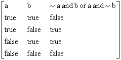

w Number theory

§ ANumNorm(a) returns the norm of the algebraic number a
Needs: Coef, MinPoly, RatNumQ
Example: ANumNorm(AlgNum(x⁴-10×x²+1,{1,-9/2,0,1/2})) Þ -1
Note: The norm of a is the product of all roots of its minimal polynomial. An algebraic number field is a finite extension field of the field of rational numbers. Within an algebraic number field is a ring of algebraic integers, which plays a role similar to the usual integers in the rational numbers. Algebraic integers and the usual “rational” integers have their similarities and differences. For example, one may lose the unique factorization of elements into products of prime powers (the Fundamental Theorem of Arithmetic). Algebraic numbers are roots of polynomial equations. A non-algebraic number is called transcendental. A good reference on algebraic number theory is Henri Cohen’s book “A Course in Computational Algebraic Number Theory.”

§ ANumTrac(a) returns the trace of the algebraic number a
Needs: Coef, MinPoly, RatNumQ
Example: ANumTrac(AlgNum(x⁴-10×x²+1,{1,-9/2,0,1/2})) Þ 2
Note: The trace of a is the sum of all roots of its minimal polynomial.

§ CarLamb(n) returns the Carmichael lambda l(n), the least universal exponent
Needs: FactList, LLcm, Totient
Example: CarLamb(5040) Þ 12
Note: A universal exponent for an integer n is an integer m such that for all k relatively prime to n, k^m º 1 (mod n).

§ CarNumQ(n) returns true if n is a Carmichael number, else false
Needs: FactList, mand
Examples: CarNumQ(561) Þ true, CarNumQ(563) Þ false
Note: A Carmichael number n is a composite integer such that for every integer b relatively prime to n, b^n-1 º 1 (mod n). For any Carmichael number n, n-1 is divisible by p-1, where p represents any of the prime factors of n.

§ CentrRem(i,j,x) returns the central remainder
Example: CentrRem(5,8,11) Þ 2
Note: The central remainder, as its name suggests, is the middle remainder in the remainder sequence (from the Euclidean algorithm) for finding a representation of a prime p as a sum of two squares.

§ cGCD(a,b) returns the GCD of complex numbers a and b
Example: cGCD(70+6×i, 150+10×i) Þ -2+2×i

§ CharPoly(a,x) gives the characteristic polynomial of the algebraic number a relative to its number field
Needs: Degree, LLcm, Resultnt, VarList
Example: CharPoly(AlgNum(x³-x+1,{2,7/3,-1}),x) Þ x³-4×x²-67×x/9+925/27
Note: CharPoly currently works only for algebraic numbers. It will be extended to work for matrices in the future.

§ ChinRem({{a₁, m₁},{a₂, m₂},…}) solves the system of congruences
k º a_i (mod m_i) for the integer k
Needs: ExtGCD, LLcm
Example: ChinRem({{1,3},{3,5},{5,8}}) Þ 120×@n1 + 13
Note: ChinRem returns the general solution. For a particular solution, set the constant @n1 to zero.

§ Divisors(n) returns the divisors of n
Needs: FactList, ListPair
Example: Divisors(147) Þ {1,2,19,38}, Divisors(541) Þ {1,541},
Divisors(3⁷) Þ {1,3,9,27,81,243,729,2187}
Note: The divisor list returned by Divisors occasionally has duplicates, and may not be sorted. A perfect number equals the sum of its proper divisors, i.e. divisors excluding itself.

§ ExtGCD(a,b) returns integers {d,{s,t}} such that d=s×a+t×b=GCD(a,b)
Needs: IsCmplxN, Quotient, VarList
Example: ExtGCD(541,547) Þ {d = 1, st = {91,-90}}
Notes: ExtGCD can be used to find the multiplicative inverse of a (mod b). For example, to solve the congruence 3×k º 4 (mod 5), multiply both sides by the mod-5 inverse (the s returned from ExtGCD(3,5)), so k = 2 × 4 = 8 is a solution. ExtGCD also works for univariate polynomials.

§ FactList(n) returns a matrix of the factors of n, with multiplicities
Needs: ReplcStr
Example: FactList(123456) Þ [[2,6][3,1][643,1]],
FactList(x²+1) Þ [[x-i,1][x+i,1]],
FactList((x+i)²) Þ [[x+i, 2]],
FactList((x+i)²/2) Þ "Error: cannot handle division at present"
Note: If xpr is an integer, FactList returns its prime factors with multiplicities. If xpr is provided as a string, the factors are found without any evaluation.

§ FundDisc(n) returns true if n is a fundamental discriminant of a quadratic number field, else returns false
Needs: Moebius
Examples: seq(FundDisc(i),i,-5,5) Þ
{false,true,true,false,false,false,false,false,false,false,true}

§ gFactor(n) returns the Gaussian factors of n
Needs: FactList, IsGPrime, Sum2Sqr
Examples: gFactor(2) Þ [[1+i,1][1-i,1]], gFactor(3) Þ [[3, 1]],
gFactor(2) Þ [[1+i,2][1-i,2]], gFactor(6) Þ [[1+i,1][1-i,1][3,1]]
Note: The returned factors may not be coprime. The result of this function may be changed in the future.

§ IsGPrime(z) returns true if z is a Gaussian prime, else false
Examples: IsGPrime(2) Þ false, (1+i)×(1-i) Þ 2, IsGPrime(1+i) Þ true

§ IsMPrime(n) returns true if n is a Mersenne prime, else returns false
Needs: LogBase, Nest
Example: seq(IsMPrime(i),i,1,8) Þ {false,false,true,false,false,false,true,false}

§ JacSymb(k,n) returns the Jacobi symbol
Needs: FactList, LegSymb
Examples: JacSymb(2,8) Þ 0, JacSymb(3,8) Þ -1
Note: JacSymb(k,n) equals LegSymb(k,n) for prime n.

§ KronSymb(m,n) returns the Kronecker symbol (m/n)
Needs: JacSymb
Example: KronSymb(2,3) Þ 1

§ LegSymb(k,n) returns the Legendre symbol
Needs: QuadResQ
Examples: LegSymb(2,3) Þ -1, LegSymb(2,7) Þ 1

§ LucasNum(n) returns the n^th Lucas number
Needs: LucasSeq
Example: LucasNum(21) Þ 24476

§ LucasSeq(p,q,L₀,L₁,n) returns the n^th term L_n of the generalized Lucas sequence with L_n+2 = p×L_n+1-q×L_n
Example: LucasSeq(1,-1,0,1,30) Þ 832040
Note: L₀ and L₁ are the initial values for the recurrence.

§ MinPoly(a,x) returns the minimal polynomial of the algebraic number a
Needs: CharPoly, ConstQ, Degree, FactList, NthCoeff, Select, SqrFree, VarList
Example: MinPoly(AlgNum(x³-x+1,{2,7/3,-1}),x) Þ 27×x³-108×x²-201×x+925
Note: The minimal polynomial of an algebraic number a is the unique irreducible monic polynomial p of smallest degree such that p(a) = 0. MinPoly currently works only for algebraic numbers. It will be extended to work for matrices in the future.

§ Moebius(n) returns the Möbius function m(n)
Needs: ReplcStr
Examples: Moebius(12) Þ 0, Moebius(12345) Þ -1, Moebius(1234567) Þ 1

§ MultMod(a,b,p) returns (a×b) (mod p) for large positive integers a, b, and p
Example: MultMod(123456789,987654321,7) Þ 3, MultMod(2⁵,3⁴,5) Þ 2
Note: MultMod is part of the MathTools Flash app; for installation instructions see the “Installation” section. Of course, you can use this function for small integers too. The full path for the MultMod function is MathTool.MultMod.

§ NFMahler(a) returns the Mahler measure of the algebraic number a
Needs: Coef, MinPoly
Example: NFMahler(AlgNum(x⁴-10×x²+1,{1,-9/2,0,1/2})) Þ Ö(2)+1
Note: The Mahler measure is widely used in the study of polynomials.

§ NFNorm(a) gives the norm of the algebraic number a relative to its number field
Needs: Degree, LLcm, Resultnt, VarList
Example: NFNorm(AlgNum(x³-x+1,{2,7/3,-1})) Þ -925/27
Note: The relative norm of a is the product of all roots of its characteristic polynomial.

§ NFTrace(a) gives the trace of the algebraic number a relative to its number field
Needs: CharPoly, Degree, VarList
Example: NFTrace(AlgNum(x³-x+1,{2,7/3,-1})) Þ 4
Note: The relative trace of a is the sum of all roots of its characteristic polynomial.

§ NxtPrime(n[,dir]) returns the next/previous prime
Examples: NxtPrime(10621) Þ 10627, NxtPrime(10621,-1) Þ 10613
Note: NxtPrime returns the next prime if dir is positive, and the previous prime if dir is negative.

§ OrderMod(a,m) returns the multiplicative (mod-m) order ord_m(a)
Needs: PowerMod, RelPrime
Examples: OrderMod(2,3) Þ 2, OrderMod(2,5) Þ 4, OrderMod(2,137) Þ 68

§ PowerMod(a,b,p) returns (a^b) (mod p) for large positive integers a, b, and p
Example: PowerMod(129140163,488281255,7) Þ 5, PowerMod(2,4⁷,5) Þ 1
Note: The modular power is perhaps the most important function in elementary number theory. PowerMod is part of the MathTools Flash app; for installation instructions see the “Installation” section. Of course, you can use this function for small integers as well. The full path for the PowerMod function is MathTool.PowerMod.

§ PowTower(x) returns the value of the infinite power tower x^x^x^… = x¥
Needs: LambertW
Example: PowTower(1.1) Þ 1.11178201104,
1.1^1.1^1.1^1.1^1.1 Þ 1.11178052653

§ Prime(n) returns the n^th prime number
Examples: Prime(10001) Þ 104743, Prime(0) Þ undef, Prime(-7) Þ undef

§ PrimePi(n) returns the number of primes less than or equal to n
Needs: LogInt, Prime
Example: PrimePi(179) Þ 41

§ Primes(n) returns the first n prime numbers
Example: Primes(11) Þ {2,3,5,7,11,13,17,19,23,29,31}

§ QuadResQ(k,p) returns true if k is a quadratic residue mod p, else false
Needs: PowerMod
Examples: QuadResQ(7,11) Þ false, QuadResQ(7,31) Þ true
Note: A number k is a quadratic residue mod p if it is relatively prime to p and there is an integer j such that k º j² (mod p).

§ RelPrime(list) returns true when all elements of list are relatively prime, else returns false
Examples: RelPrime({5,7}) Þ true, RelPrime({2,4}) Þ false,
RelPrime({x-2,x³+2×x²-x-2}) Þ true
Notes: RelPrime works for numbers and univariate polynomials. The probability that n integers chosen at random are relatively prime is 1/z(n), where z(n) is the zeta function. The Fermat numbers 2^2^n+1 are relatively prime.

§ RndPrime(n) returns a random prime number in [1,n]
Example: RandSeed 0:RndPrime(10⁹) Þ 951898333

§ SqrtModP(a,p) returns the smallest nonnegative square-root of a (mod p)
Needs: JacSymb, PowerMod
Examples: SqrtModP(123456,987) Þ 360, SqrtModP(1234567,987) Þ {}
Note: SqrtModP uses Shanks’ method. It returns {} if there is no square-root.

§ SqrtNOMP(p) returns a square-root of -1 mod p
Needs: JacSymb, PowerMod, Sort
Example: SqrtNOMP(1741) Þ 59

§ Sum2Sqr(p) returns {a,b} where p = a²+b²
Needs: CentrRem, SqrtNOMP
Examples: Sum2Sqr(5) Þ {1,2}, Sum2Sqr(103841) Þ {104,305}
Note: Sum2Sqr uses Smith’s algorithm to find {a,b}.

§ SumOfSqN(d,n) returns the number of representations r_d(n) of n as a sum of d squares of integers
Needs: Divisors, DivSigma, FactList, IntExp, JacSymb, Moebius
Examples: SumOfSqN(2,5) Þ 8, SumOfSqN(3,4) Þ 6,
SumOfSqN(7,3) Þ 280, SumOfSqN(5,217) Þ 27840

§ Totient(n) returns the Euler j(n) function, which is the number of positive integers less than n that are relatively prime to n
Needs: FactList
Examples: Totient(143055667) Þ 142782138, Totient(17¹⁰⁰) Þ 1043669997…
Note: The Euler totient function is a multiplicative function, which is a function f: ® such that whenever gcd(i,j) = 1, f(i×j) = f(i)×f(j), so that one can obtain f(n) by multiplying f(p^k), where p^k is a prime power from the factorization of n. For all n greater than 1, the value of j(n) lies between 1 and n-1, inclusive. j(n) = n-1 iff n is prime. Also, for n > 2, j(n) is even.

w Optimization

§ LagrMult(f(x,y,…),{cond1,cond2,…},{x,y,…}) finds extrema for f(x,y,…) subject to the conditions {cond1=0, cond2=0, …}
Needs: list2eqn
Example: LagrMult(x²+y²,{x²+y-1},{x,y}) Þ x = Ö(2)/2 and y = 1/2 and …
Note: If you want LagrMult to return the maximum/minimum values of f(x,y,…) in addition to the values of x,y,…, open the function in the Program Editor and delete the “Return hh” line. The extrema returned may be local or global extrema. You can use the Hessian to determine the type of extremum.

§ Minimize({f, constraints},{vars, start},{{opt1,val1},…}) finds a minimum of the objective function f subject to the given constraints
Needs: FuncEval, mand
Examples: RandSeed 0: Minimize({x^2+(y-1/2)^2, y>=0, y>=x+1},
{{x,y},{5,5}},{{“MaxIterations”,2}})
Note: Minimize is a program (instead of a function) so that the user can get an overview of the progress. It currently uses the method of simulated annealing. Minimize is experimental and is generally slow, especially with constraints.

§ Simplex(obj,cmat) returns the minimum for the linear programming problem with the objective function given by obj and the constraints given by cmat
Needs: ListSubt, Select, SimpStep, Sort
Example: Minimize f = 5×x-3×y-8×z subject to the constraints
{2×x+5×y-z£1, -2×x-12×y+3×z£9, -3×x-8×y+2×z£4, x³0, y³0, z³0}
Simplex({5,-3,-8,0,0,0,-1,0},
[[2,5,-1,1,0,0,0,1][-2,-12,3,0,1,0,0,9][-3,-8,2,0,0,1,0,4]]) Þ
{-121, vars = {0,3,14,0,3,0}}
Note: There are two widely used solution techniques for linear programming: simplex methods and interior point methods. While simplex methods move from vertex to vertex along the edges of the boundary of the feasible region, interior point methods visit points within the interior of the feasible region. The Simplex function currently uses the tableau form of the simplex method. The input list is obtained in the above example by setting 5×x-3×y-8×z-f = 0, so that f has a coefficient of -1. You can also enter a shortened form of the list as {5,-3,-8}. The rows in cmat give the coefficients of the original variables and the “slack” variables in the constraints. There is a slack variable for each inequality constraint. A slack variable allows you to turn an inequality constraint into an equality constraint. So, for example, the first constraint in the above example would become 2×x+5×y-z+s₁ = 1. The final result displays the minimum of f and the values of the original and slack variables at the minimum. So, for the above example, f has a minimum at -121, where {x=0, y=3, z=14, s₁=0, s₂=3, s₃=0}. To find the maximum rather than the minimum, simply find the minimum of –f and flip the sign of f in the result.

§ SimpStep(obj,mat,bvars) does pivoting for a single step of the simplex method and gives the tableau for the next basic feasible solution with the specified basic variables bvars
Needs: ListSubt
Example: SimpStep({5,-3,-8,0,0,0,-1,0}, [[2,5,-1,1,0,0,0,1][-2,-12,3,0,1,0,0,9]
[-3,-8,2,0,0,1,0,4]], {3,4,5}) Þ
[[-3/2,-4,1,0,0,1/2,0,2][1/2,1,0,1,0,1/2,0,3]
[5/2,0,0,0,1,-3/2,0,3][-7,-35,0,0,0,4,1,16]]
Note: The rows represent the results for {bvars[1],bvars[2],…,bvars[n],f}, where f is the objective function. Non-basic variables (the variables not in bvars, in this case {1,2,6}) are assumed to be zero, so that one can read off the result for each basic variable by looking at the number in the last column.

w Pattern-matching

§ FreeQ(expression1,expression2) returns true if expression1 is free of expression2, else returns false
Needs: mand
Examples: FreeQ(y^(a×x²+b),x) Þ false, FreeQ(ln(cos(x)),y) Þ true,
FreeQ({a,b^2×x,c,d²},2×x) Þ false, FreeQ(x²,"cos") Þ true,
FreeQ(cos(x)²,"cos") Þ false
Note: Please see MatchQ entry for a note on auto-simplification.

§ MatchQ(expression,form) returns true if the structure of expression matches that of form, else returns false
Needs: mand
Examples: MatchQ(2,x) Þ false, MatchQ(2,x_) Þ true, MatchQ(a²,x_) Þ true,
MatchQ(a²,x_+y_) Þ false, MatchQ(a^x×f(x),2^x×f(x)) Þ false,
MatchQ(2^x×f(x), a^x×f(x)) Þ false, MatchQ(2^x×f(x), a_^x×f(x)) Þ true,
MatchQ(a(b,c),d(e,f,g)) Þ false, MatchQ(a(b,c),d(e,f)) Þ false,
MatchQ(a_(b_,c_),d_(e_,f_)) Þ true
Note: The AMS performs some auto-simplification before MatchQ can use the expression, so for example MatchQ(x+x,a_+b_) Þ false, because x+x is simplified to 2×x. This can affect the form as well. Here is another example: MatchQ(x²×y(n),a_×f_(n)) Þ false, while MatchQ(x²×c(n),a_×f_(n)) Þ true. This auto-simplification can be good or bad, depending on the context. In general, I would suggest trying expressions and forms out on the home screen to see how they are auto-simplified before using them in MatchQ. Also, until I implement default values for MatchQ, x will not match a_^n_ ; this is because the structure does not match exactly unless you use a default value of 1 for powers.

w Special Functions

§ AiryAi(x) returns the Airy function Ai(x) for real x
Needs: Gamma
Examples: AiryAi(0.1) Þ 0.329203129944, AiryAi(7.3) Þ 0.000000332514

§ AiryBi(x) returns the Airy function Bi(x) for real x
Needs: Gamma
Examples: AiryBi(-5.2) Þ -0.275027044184, AiryBi(9.5) Þ 96892265.5804

§ BellNum(n) returns the n^th Bell number
Needs: BellPoly
Example: seq(BellNum(i),i,0,6) Þ {1,1,2,5,15,52,203}

§ BellPoly(n,x) returns the n^th Bell polynomial
Needs: BellNum
Example: BellPoly(5,x) Þ x⁵+10×x⁴+25×x³+15×x²+x
Note: BellPoly(n,1) returns the n^th Bell number.

§ BernNum(n) returns the n^th Bernoulli number B_n
Needs: Zeta
Example: seq(BernNum(i),i,1,6) Þ {-1/2,1/6,0,-1/30,0,1/42}

§ BernPoly(n,x) returns the n^th Bernoulli polynomial B_n(x)
Needs: IsCmplxN, Zeta
Example: BernPoly(3,x) Þ x³-3×x²/2+x/2

§ BesselI(n,z) returns the n^th modified Bessel function of the first kind I_n(z)
Needs: BesselJ
Examples: BesselI(3/2,x) Þ Ö(2)×((x-1)×(e^x)²+x+1)/(2×Ö(p)×x^3/2×e^x),
BesselI(0.92,0.35) Þ 0.210999194087-2.2083340901E-16×i
Note: Please see the note in the help entry for BesselJ.

§ BesselJ(n,z) returns the n^th Bessel function of the first kind J_n(z)
Needs: Gamma, IsCmplxN
Examples: BesselJ(3/2,x) Þ Ö(2)×sin(x)/(Ö(p)×x^3/2)-Ö(2)×cos(x)/(Ö(p)×Ö(x)),
BesselJ(2,1/2) Þ 0.030604023459, BesselJ(51/2,1.×π) Þ 0.
Note: Symbolic results from BesselJ for half-integer n may give incorrect results for subsequent floating point evaluation because of catastrophic cancellation. Do comDenom(symbresult|x=«value», q) and then approximate it, or calculate the numeric result directly (see the last example above).

§ BesselK(n,z) returns the n^th modified Bessel function of the second kind K_n(z)
Needs: BesselI
Example: BesselK(5/2,x) Þ
Ö(p)×Ö(2)/(2×Ö(x)×e^x)+3×Ö(p)×Ö(2)/(2×x^3/2×e^x)+3×Ö(p)×Ö(2)/(2×x^5/2×e^x)
Note: Please see the note in the help entry for BesselJ.

§ BesselY(n,z) returns the n^th Bessel function of the second kind Y_n(z)
Needs: BesselJ
Example: BesselY(3/2,x) Þ -Ö(2)×cos(x)/(Ö(p)×x^3/2)-Ö(2)×sin(x)/(Ö(p)×Ö(x)),
BesselY(1,10.3) Þ 0.24706994
Note: Please see the note in the help entry for BesselJ.

§ Beta(p,q) returns the beta function B(p,q)
Needs: Gamma
Example: Beta(1/2,2) Þ 4/3
Note: The (complete) beta function is symmetric in its arguments, that is,
B(p,q) = B(q,p).

§ Catalan(n) returns the n^th Catalan number
Example: seq(Catalan(i),i,1,6) Þ {1,2,5,14,42,132}

§ ChebyT(n,x) returns the n^th Chebyshev polynomial of the first kind T_n(x)
Needs: Gamma
Example: ChebyT(5,x) Þ 16×x⁵-20×x³+5×x, ChebyT(n,0) Þ cos(n×p)/2

§ ChebyU(n,x) returns the n^th Chebyshev polynomial of the second kind U_n(x)
Needs: Gamma
Example: ChebyU(6,x) Þ 64×x⁶-80×x⁴+24×x²-1, ChebyU(n,1) Þ n+1

§ Clebsch(j₁,m₁,j₂,m₂,j,m) returns the Clebsch-Gordan coefficient
Needs: ReplcFac
Examples: Clebsch(1/2,1/2,1/2,-1/2,1,0) Þ Ö(2)/2,
Clebsch(1,1,1,1/2,2,3/2) Þ Ö(105)/12

§ Cyclotom(n,x) returns the n^th cyclotomic polynomial
Needs: RelPrime
Example: Cyclotom(6,x) Þ x²-x+1
Note: The n^th cyclotomic polynomial is the minimal polynomial of the primitive n^th root of unity and is irreducible over with degree j(n), where j(n) is the Euler totient function.

§ DblFact(n) returns the double factorial n!!
Needs: IsCmplxN
Example: DblFact(14) Þ 645120, DblFact(2.1) Þ 2.10479089216

§ DivSigma(n,k) returns the sum s_k(n) of k^th powers of the divisors of n
Needs: FactList
Examples: DivSigma(111,0) Þ 4, DivSigma(111,1) Þ 152,
DivSigma(111,2) Þ 13700
Note: As special cases, DivSigma(n,0) returns the number of divisors and DivSigma(n,1) returns the sum of the divisors. The divisors in the example above are {1,3,37,111}. A perfect number equals the sum of its proper divisors, i.e. divisors excluding itself.

§ Erf(x) returns the error function
Needs: Erfi
Examples: Erf(0.5) Þ 0.520499877813, Erf(3.7) Þ 0.999999832845,
Erf(i) Þ 1.6504257588×i
Note: The n^th derivative of erf(x) involves the n-1^th Hermite polynomial.

§ Erfc(x) returns the complementary error function
Needs: Erf
Example: Erfc(0.5) Þ 0.479500122187

§ Erfi(z) returns the imaginary error function erf(i×z)/i
Needs: Erf, Hypg1F1
Examples: Erfi(1) Þ 1.6504257588, Erfi(-i) Þ -0.84270079295×i

§ Euler(n,x) returns the n^th Euler polynomial
Needs: BernPoly, IsCmplxN
Example: Euler(4,x) Þ x⁴-2×x³+x
Note: The n^th Euler number is given by 2ⁿ×Euler(n,1/2).

§ ExpIntE(n,x) returns the exponential integral E_n(x)
Needs: IncGamma
Examples: ExpIntE(-1,z) Þ ((z+1)×e^-z)/z², ExpIntE(8,0) Þ 1/7

§ ExpIntEi(x) returns the exponential integral Ei(x)
Examples: ExpIntEi(2.3) Þ 6.15438079133,
ExpIntEi(98.1) Þ 4.14110745294E40,
ExpIntEi(-5) Þ -0.001148295591,
ExpIntEi(-6) Þ -0.000360082452

§ FibNum(n) returns the n^th Fibonacci number F_n
Examples: seq(FibNum(i),i,1,6) Þ {1,1,2,3,5,8},
FibNum(2000) Þ <418-digit integer> (takes about 29 seconds),
FibNum(2000.) Þ 4.22469633342E417 (takes about 0.21 seconds)
Note: The ratios of alternate Fibonacci numbers are said to measure the fraction of a turn between successive leaves on the stalk of a plant. Also, the number of petals on flowers are said to be Fibonacci numbers. (See MathWorld entry.) FibNum uses a combination of the Binet formula and the Q-matrix method.

§ FibPoly(n,x) returns the n^th Fibonacci polynomial F_n(x)
Example: FibPoly(7,x) Þ x⁶+5×x⁴+6×x²+1
Note: Fibonacci polynomials are used in a variety of fields, such as cryptography and number theory.

§ FresnelC(x) returns the Fresnel cosine integral C(x) for real x
Examples: FresnelC(0.78) Þ 0.748357308436,
FresnelC(6.4) Þ 0.549604555704, FresnelC(0) Þ 0

§ FresnelS(x) returns the Fresnel sine integral S(x) for real x
Needs: FresnelC
Examples: FresnelS(1.1) Þ 0.625062823934,
FresnelS(13.7) Þ 0.479484940352, FresnelS(0) Þ 0

§ Gamma(z) returns the gamma function G(z)
Needs: DblFact, IsCmplxN
Examples: Gamma(11/2) Þ 945×Ö(p)/32, Gamma(1/3) Þ 2.67893853471,
Gamma(1+5×i) Þ -0.001699664494-0.001358519418×i
Note: The gamma function generalizes the factorial function from the natural numbers to the complex plane. However, it is not a unique solution to the problem of extending x! into complex values of x. Other solutions are of the form f(x) = G(x)×g(x), where g(x) is an arbitrary periodic function with period 1.

§ Gegenbau(n,m,x) returns the n^th Gegenbauer polynomial for the parameter m
Needs: Gamma, IsCmplxN
Example: Gegenbau(4,2,x) Þ 80×x⁴-48×x²+3

§ Hermite(n,x) returns the n^th Hermite polynomial H_n(x)
Example: Hermite(4,x) Þ 16×x⁴-48×x²+12, Hermite(n,0) Þ 2ⁿ×Ö(p)/(-n/2-1/2)!,
Hermite(100,1) Þ -1448706729…, Hermite(10,-3) Þ -3093984,
Hermite(-1,3) Þ 0.15863565
Note: For any given interval (a,b) there is always a Hermite polynomial that has a zero in the interval.

§ Hypg1F1(a,c,z) returns Kummer’s confluent hypergeometric function ₁F₁(a;c;z)
Needs: Gamma
Examples: 1/Ö(p)×Hypg1F1(1/2,3/2,-(1/2)²) Þ 0.520499877813,
Hypg1F1(1,2,1) Þ e-1, Hypg1F1(3,1,x) Þ (x²/2+2×x+1)×e^x,
Hypg1F1(-2,3/2,x) Þ ((4×x²-20×x+15)/15), Hypg1F1(a,a,x) Þ e^x,
expand(Hypg1F1(-2,b,x),x) Þ x²/(b×(b+1))-2×x/b+1,
Note: 1/Ö(p)×Hypg1F1(1/2,3/2,-x²) gives the error function erf(x).

§ Hypg2F1(a,b,c,z) returns Gauss’ hypergeometric function ₂F₁(a,b;c;z)
Needs: ChebyT, Gamma, Gegenbau, Jacobi, Legendre
Examples: Hypg2F1(1/2,1/2,3/2,x²) Þ sin^-1(x)/x, Hypg2F1(1,1,1,-x) Þ 1/(x+1),
Hypg2F1(1,1,2,1-x) Þ ln(x)/(x-1),
Hypg2F1(-3,3,-5,z) Þ z³+9×z²/5+9×z/5+1,
Hypg2F1(1/3,1/3,4/3,1/2) Þ 1.05285157425,

§ HypgPFQ({a₁,a₂,…,a_p},{b₁,b₂,…,b_q},z) returns the generalized hypergeometric function _pF_q(a;b;z)
Needs: Gamma, Hypg1F1, Hypg2F1
Examples: HypgPFQ({},{},x) Þ e^x, HypgPFQ({},{1/2},-x²/4) Þ cos(x)

§ HZeta(n,z) returns the Hurwitz zeta function
Needs: Psi
Examples: HZeta(4,1/2) Þ p⁴/6, HZeta(0,-x/2) Þ (x+1)/2,
HZeta(2,1/4) Þ 8×çatalan+p², HZeta(n,3) Þ -2^-n+z(n)-1,
HZeta(-3,1/4) Þ -7/15360, HZeta(4.2,5) Þ 0.002471293458

§ IncBeta(z,a,b) returns the incomplete beta function B_z(a,b)
Needs: Beta, Pochhamm
Examples: IncBeta(1,-3/2,2) Þ 4/3, IncBeta(5,4,9) Þ 1142738125/396

§ IncGamma(n,x) returns the incomplete gamma function G(n,x)
Needs: ExpIntEi, Gamma, IsCmplxN, Pochhamm
Examples: IncGamma(2,z) Þ (z+1)×e^-z, IncGamma(11,1) Þ 9864101×e^-1,
IncGamma(1.2,5.8) Þ 0.004435405791, IncGamma(n,1) Þ G(n,1)

§ InvErf(x) returns the inverse erf^-1(x) of the error function
Example: InvErf(0.013) Þ 0.011521459812, Erf(0.011521459812) Þ 0.013

§ InvErfc(x) returns the inverse erfc^-1(x) of the complementary error function
Needs: InvErf
Example: InvErfc(1/2) Þ 0.476936276204, Erfc(0.476936276204) Þ 0.5

§ Jacobi(n,a,b,x) returns the Jacobi polynomial
Needs: Gamma, IsCmplxN
Examples: Jacobi(3,2,2,1) Þ 10, Jacobi(3,2,1,x) Þ (21×x³+7×x²-7×x-1)/2
Note: Jacobi polynomials are the most general orthogonal polynomials for x in the interval [-1, 1].

§ KDelta({n₁,n₂,…}) returns 1 if n₁=n₂=…, else returns 0
Examples: KDelta({0,0,1,0}) Þ 0, KDelta({0,0,0,0}) Þ 1,
KDelta({1,1,1}) Þ 1, KDelta({a,1}) Þ 0, KDelta({a,a}) Þ 1

§ Laguerre({n,k},x) returns the associated Laguerre polynomial
Examples: Laguerre(3,x) Þ (-x³+9×x²-18×x+6)/6, Laguerre(n,0) Þ 1,
Laguerre({3,1},x) Þ (-x³+12×x²-36×x+24)/6
Note: If you give an integer n as the first argument, you get the ordinary Laguerre polynomial L_n(x). Laguerre polynomials appear as eigenfunctions of the hydrogen atom in quantum mechanics.

§ LambertW(x) returns the principal branch of the Lambert W function
Example: LambertW(2/3×e^2/3) Þ 2/3,
LambertW(0.12) Þ 0.10774299816228 [approximately 0.68 seconds]
(solving the equation without an initial guess takes about 8 seconds)
Note: The Lambert W function is defined by x = W(x)×e^W(x)

§ Legendre({n,m},x) returns the associated Legendre function of the first kind
Needs: Gamma, ReplcStr
Examples: Legendre(3,x) Þ (5×x³)/2-(3×x)/2, Legendre(10,0) Þ -63/256,
Legendre({3,1},x) Þ (15×x²×Ö(1-x²))/2-(3×Ö(1-x²))/2
Note: The returned function may have an extra factor of (-1)^m. If you give an integer n as the first argument, you get the ordinary Legendre polynomial P_n(x). Because of the rather low value of the maximum representable number on these devices, a bug can crop up when trying to evaluate the Legendre polynomials for large n, e.g. Legendre(1000,0) incorrectly returns zero.

§ Legendr2({n,m},x) returns the associated Legendre function of the second kind
Needs: Gamma, Legendre
Examples: Legendr2(70,0) Þ 0, Legendr2(1/2,0) Þ -0.847213084794,
Legendr2(0,x) Þ ln(x+1)/2-ln(-(x-1))/2
Note: If you give an integer n as the first argument, you get the ordinary Legendre polynomial Q_n(x). Please also see the notes for Legendre.

§ LogInt(x) returns the logarithmic integral li(x)
Needs: ExpIntEi
Example: LogInt(0.1) Þ -0.032389789593

§ LucasNum(n) returns the n^th Lucas number
Needs: LucasSeq
Example: LucasNum(21) Þ 24476

§ LucasSeq(p,q,L₀,L₁,n) returns the n^th term L_n of the generalized Lucas sequence with L_n+2 = p×L_n+1-q×L_n
Example: LucasSeq(1,-1,0,1,30) Þ 832040
Note: L₀ and L₁ are the initial values for the recurrence.

§ Moebius(n) returns the Möbius function m(n)
Needs: ReplcStr
Examples: Moebius(12) Þ 0, Moebius(12345) Þ -1, Moebius(1234567) Þ 1

§ Multinom(list) returns the number of ways of partitioning N=sum(list) objects into m=dim(list) sets of sizes list[i]
Example: Multinom({a,b,c}) Þ (a+b+c)!/(a!×b!×c!)

§ PellNum(n) returns the n^th Pell number
Example: seq(PellNum(i),i,1,6) Þ {1,2,5,12,29,70}
Note: The Pell numbers are the U_n’s in the Lucas sequence.

§ Pochhamm(a,n) returns the Pochhammer symbol (a)_n
Needs: Gamma
Example: Pochhamm(x,3) Þ x×(x+1)×(x+2)

§ Polylog(n,z) returns the polylogarithm Li_n(z)
Needs: FuncEval, Gamma, HZeta, IsCmplxN, Psi, Zeta
Examples: Polylog(-1,x) Þ x/(x-1)², Polylog(2,-1) Þ -p²/12,
Polylog(2,-2) Þ -1.43674636688

§ Psi(n,z) returns the polygamma function

Needs: BernNum, Zeta
Examples: Psi(3,1/2) Þ p⁴,
Psi(0,i) Þ 0.094650320623+2.07667404747×i,
Psi(2,6.38) Þ -0.028717418078,
Psi(0,11/3) Þ -g - (3×ln(3))/2 + (p×Ö(3))/6 + 99/40,
Psi(13,2) Þ (2048×p¹⁴)/3 - 6227020800
Note: Psi(0,z) returns the digamma function . Psi(n,z) is the (n+1)^th logarithmic derivative of the gamma function G(z). The g returned in results is the Euler gamma constant g » 0.57721566490153, sometimes also called the Euler-Mascheroni constant.

§ RegGamma(a,x) returns the regularized incomplete gamma function Q(a,x)
Needs: Erfc, Gamma, IncGamma, Pochhamm
Examples: RegGamma(0,x) Þ 0, RegGamma(-91,x) Þ 0,
RegGamma(3,x) Þ (x²/2+x+1)×e^-x

§ SBesselH(k,n,x) returns the spherical Bessel function for k=1 or k=2
Examples: SBesselH(1,1,x) Þ -((x+i)×e^i×x)/x²,
SBesselH(2,1,x) Þ -((x+-i)×e^-i×x)/x²

§ SBesselI(n,x) returns the modified spherical Bessel function
Example: SBesselI(n,x) Þ (e^-x×((x-1)×e^2×x+x+1))/(2×x²)

§ SBesselJ(n,x) returns the spherical Bessel function
Example: SBesselJ(1,x) Þ -(x×cos(x)-sin(x))/x²

§ SBesselK(n,x) returns the modified spherical Bessel function
Example: SBesselK(1,x) Þ ((x+1)×e^-x)/x²

§ SBesselN(n,x) returns the spherical Bessel function
Example: SBesselN(1,x) Þ -cos(x)/x²-sin(x)/x

§ SinInt(x) returns the sine integral function Si(x) for real x
Examples: SinInt(0.007) Þ 0.00699998, SinInt(0.1) Þ 0.0999445,
SinInt(-0.1) Þ -0.0999445, SinInt(18.2) Þ 1.529091

§ SphrHarm(l,m,q,j) returns the spherical harmonic Y_l^m(q,j)
Needs: Legendre
Example: SphrHarm(2,0,q,f) Þ ((3×(cos(q))²-1)×Ö(5))/(4×Ö(p))

§ StirNum1(n,k) returns the Stirling number of the first kind
Needs: StirNum2
Example: StirNum1(5,3) Þ 35
Note: (-1)^n-k×StirNum1(n,k) gives the number of permutations of n items that have exactly k cycles.

§ StirNum2(n,k) returns the Stirling cycle number
Example: StirNum2(11,4) Þ 145750
Note: The Stirling cycle number gives the number of ways one can partition an n-element set into k non-empty subsets. It also occurs in summing powers of integers.

§ StruveH(n,z) returns the Struve function H_n(z)
Needs: BesselJ, BesselY, Pochhamm
Examples: StruveH(1/2,0) Þ 0,
StruveH(1/2,x) Þ Ö(2)×(Ö(p)×Ö(x))-Ö(2)×cos(x)/(Ö(p)×Ö(x))
Note: This function currently works mainly only for half-integer n.

§ Subfact(n) returns the number of permutations of n objects which leave none of them in the same place
Needs: IsCmplxN
Example: Subfact(20) Þ 895014631192902121

§ Totient(n) returns the Euler j(n) function, which is the number of positive integers less than n that are relatively prime to n
Needs: FactList
Examples: Totient(143055667) Þ 142782138, Totient(17¹⁰⁰) Þ 1043669997…

§ Wigner3j(j₁,m₁,j₂,m₂,j₃,m₃) returns the Wigner 3-j symbol
Needs: Clebsch
Example: Wigner3j(2,1,5/2,-3/2,1/2,1/2) Þ Ö(30)/15

§ Zeta(z) returns the Riemann zeta function z(z)
Examples: Zeta(2) Þ p²/6, Zeta(1-i) Þ 0.00330022-0.418155×i,
Zeta(1/2+7×i) Þ 1.02143 + 0.396189×i, Zeta(k) Þ z(k)
Notes: The Riemann zeta function has a central role in number theory. It also appears in integration and summation. For small approximate values, Zeta seems to have an error of 10^-9 or less. For large negative values, the error may be significant due to the limited precision on these calculators, even though most of the digits returned are correct. For example, the error for Zeta(-98.4) is approximately 4.17×10⁶², and the error for Zeta(-251.189) is approximately 3.99×10²⁸¹. Zeta seems quite accurate for large positive values, where the zeta function approaches 1. Two other commonly used sums of reciprocal powers of integers can be related to the zeta function: ,

§ ZetaPrim(z) returns the first derivative of the zeta function z'(z)
Needs: BernNum
Examples: ZetaPrim(2) Þ -0.937548, ZetaPrim(i) Þ 0.0834062-0.506847×i,
ZetaPrim(-1) Þ 1/12-ln(glaisher),
ZetaPrim(-1.0) Þ -0.165421143696,
ZetaPrim(k) Þ z'(k)
Note: The symbol ‘glaisher’ returned in results represents the Glaisher-Kinkelin constant A » 1.2824271291006, and satisfies the equation ln(A) = 1/12 - z'(-1). It appears in sums and integrals of some special functions.

w Statistics

§ CDF(StatDist("DistributionName",parameters), x) returns the distribution probability between -¥ and x for the given distribution and parameters
Needs: Erf, Erfc, Gamma, IncGamma
Examples: CDF(statdist("Cauchy",{1,2}),0.7) Þ 0.452606857723,
CDF(statdist("Cauchy",{1,2}),x) Þ tan^-1((x-1)/2)/p+1/2,
CDF(statdist("Chi^2",{0.3}),0.11) Þ 0.688767224365,
CDF(statdist("Exponential",{0.83}),0.04) Þ 0.032654928773,
CDF(statdist("Gamma",{1/2,1/4}),2) Þ 0.999936657516,
CDF(statdist("Gamma",{1/2,1/4}),x) Þ 1-G(1/2,4×x)/Ö(p),
CDF(statdist("Hypergeometric",{2,3,7}),1/3) Þ 2/7,
CDF(statdist("Laplace",{0.96,0.32}),0.5) Þ 0.118760409548,
CDF(statdist("Logistic",{2.5,1}),4) Þ 0.817574476194,
CDF(statdist("Normal",{0,1}),0.2) Þ 0.579259709439,
CDF(statdist("Poisson",{4/3}),9/4) Þ 29×e^-4/3/9

§ CentrMom(list,r) returns the r^th central moment of list
Example: CentrMom({a,b},2) Þ (a-b)²/4

§ Freq(list) returns the distinct elements of list with their frequencies
Needs: Sort
Example: Freq({a,b,b,c,a}) Þ [[a,b,c][2,2,1]]

§ GeomMean(list) returns the geometric mean of list
Example: GeomMean({a,b}) Þ Ö(a×b)

§ HarmMean(list) returns the harmonic mean of list
Example: HarmMean({a,b}) Þ 2×a×b/(a+b)

§ IntQuant(list,q) returns the q^th interpolated quantile of a probability distribution
Needs: Sort
Example: IntQuant({a,b,c,d},0.75) Þ c
Note: The quantile is obtained from a linear interpolation of list. IntQuant can be used to find quartiles, deciles, etc.

§ Kurtosis(list) returns the Pearson kurtosis coefficient for list
Needs: CentrMom, PStdDev
Example: Kurtosis({a,b,c}) Þ 3/2

§ MeanDev(list) returns the mean absolute deviation about the mean for list
Example: MeanDev({a,b}) Þ |a-b|/2

§ MedDev(list) returns the median absolute deviation about the median for list
Example: MedDev({2,3}) Þ 1/2

§ Mode(list) returns the most frequent element(s) of list
Needs: Freq
Example: Mode({a,b,b,c,a}) Þ {a,b}

§ MovAvg(list,n) smooths list using an n-point moving average
Example: MovAvg({a,b,c},2) Þ {(a+b)/2,(b+c)/2}

§ MovMed(list,n) smooths list using a span-n moving median
Example: MovMed({3,7,1,0,5},3) Þ {3,1,1}

§ PDF(StatDist("DistributionName",parameters), x) returns the probability density function at x for the given distribution and parameters
Needs: Gamma
Examples: PDF(statdist("Cauchy",{0.22,0.81}),0.75) Þ 0.275166497128,
PDF(statdist("Chi^2",{1/2}),0.4) Þ 0.377535275007,
PDF(statdist("Exponential",{5}),1/4) Þ 5×e^-5/4,
PDF(statdist("Exponential",{a}),x) Þ a×e^-a×x,
PDF(statdist("FRatio",{0.03,0.14}),0.9) Þ 0.013213046749,
PDF(statdist("Gamma",{0.3,0.72}),0.45) Þ 0.178995053492,
PDF(statdist("Hypergeometric",{4,5,8}),3) Þ 3/7,
PDF(statdist("Laplace",{0.61,0.05}),0.37) Þ 0.08229747049,
PDF(statdist("Logistic",{0.14,0.8}),5.7) Þ 0.001195999788,
PDF(statdist("Normal",{0,1}),x) Þ Ö(2)×/(2×Ö(p)),
PDF(statdist("Normal",{0.2,3}),1/3) Þ 0.132849485949,
PDF(statdist("Poisson",{9}),2) Þ 81×e^-9/2,
PDF(statdist("StudentT",{0.66}),0.5) Þ 0.222461859264,
PDF(statdist("StudentT",{3}),x) Þ 6×Ö(3)/(p×(x²+3)²)

§ PStdDev(list) returns the most likely estimate for the population standard deviation of list
Example: stdDev({a,b}) Þ |a-b|×Ö(2)/2, PStdDev({a,b}) Þ |a-b|/2

§ Quantile(list,q) returns the q^th quantile
Needs: Sort
Example: Quantile({a,b},0.6) Þ b

§ Random(StatDist("DistributionName",parameters)) returns a pseudorandom number using the given statistical distribution
Examples: RandSeed 0:Random(statdist("Bernoulli",{14})) Þ 1,
RandSeed 0:Random(statdist("Beta",{2.4,-0.11})) Þ 0.304489,
RandSeed 0:Random(statdist("Binomial",{4,2/3})) Þ 2,
RandSeed 0:Random(statdist("Cauchy",{-3/2,4})) Þ 20.8374,
RandSeed 0:Random(statdist("Chi^2",{1})) Þ 0.0603222,
RandSeed 0:Random(statdist("DiscreteUniform",{-21,37})) Þ 34,
RandSeed 0:Random(statdist("Gamma",{0.5,0.5})) Þ 0.0150806,
RandSeed 0:Random(statdist("Geometric",{0.027})) Þ 2,
RandSeed 0:Random(statdist("Hypergeometric",{5,3,10})) Þ 3,
RandSeed 0:Random(statdist("Logistic",{0.5,0.5})) Þ 1.90859,
RandSeed 0:Random(statdist("LogNormal",{0.5,0.5})) Þ 1.90195,
RandSeed 0:Random(statdist("Normal",{1,0.4})) Þ 2.01958,
RandSeed 0:Random(statdist("Poisson",{3.2})) Þ 6,
RandSeed 0:Random(statdist("Uniform",{})) Þ 0.943597,
RandSeed 0:Random(statdist("Uniform",{-13,21.2})) Þ 19.2710

§ RMS(list) returns the root-mean-square of list
Example: RMS({a,b,c}) Þ Ö(a²+b²+c²)/3

§ Skewness(list) returns the skewness coefficient for list
Needs: CentrMom, PStdDev
Examples: Skewness({a,b}) Þ 0, Skewness({1,2,2.1}) Þ -0.685667537489

§ TrimMean(list,a) returns the a-trimmed mean
Needs: Sort
Examples: TrimMean({a,b,c},1/10) Þ (7×a+10×b+7×c)/24,
TrimMean({2,8,4},1/10) Þ 55/12
Note: The trimmed mean is equal to the arithmetic mean when a=0.

w Strings

§ nChars(str,chr) returns the number of occurrences of chr in the string str
Examples: nChars("mathtools","o") Þ 2, nChars("mathematics","ma") Þ 2

§ RepChars(chars,n) returns a string with chars repeated n times
Example: RepChars("math",3) Þ "mathmathmath"

§ ReplcStr(str1,str2,str3) replaces occurrences of the string str2 with str3 in str1
Example: ReplcStr("aububu","ub","qq") Þ "aqqqqu"

§ Str2Chrs(str) returns a list of the characters in the string str
Example: Str2Chrs("a bc") Þ {"a"," ","b","c"}

§ StrCount(str,substr) is an alternative function that returns the number of occurrences of substr in str
Example: StrCount("more & more","or") Þ 2

w Summation and Series

§ Aitken(list) accelerates series with Aitken’s d² method and returns {sn, delta}
Example: Aitken(seq((-1)^k/(2×k+1),k,0,10)) Þ {0.785459904732, 0.00014619883}
Notes: The first few terms of the series are given in ‘list’. For example, to accelerate the series å(x(i),i,a,b), one could use seq(x(i),i,a,a+10). ‘sn’ is the last accelerated sum, and ‘delta’ is the difference between the last two sums.

§ EMSum(x(i),i,a,expstart,b,exporder) returns an asymptotic (Euler-Maclaurin) expansion for the sum å(x(i),i,a,b)
Examples: å(1/(2^k),k,0,¥) Þ 2,
EMSum(1/(2^k),k,0,1,¥,5.) Þ 2.0000000000047,
å(e^{1/x^2}-1,x,1,¥) Þ å(e^{1/x^2}-1,x,1,¥) [unevaluated],
EMSum(e^{1/x^2}-1,x,1,5,¥,4.) Þ 2.40744653864
Note: expstart is the start of the expansion and exporder is the expansion order. The formula was taken from the “Handbook of Mathematical Functions”, by Abramowitz and Stegun.

§ Gosper(xpr,var,low,up) does hypergeometric summation å(xpr,var,low,up)
Examples: Gosper(k×k!,k,0,n-1) Þ n!-1,
Gosper(4^k/nCr(2×k,k),k,0,n-1) Þ (2×n-1)×(n!)²×4ⁿ/(3×(2×n)!)+1/3
Notes: Gosper returns "No solution found" if the requested sum cannot be summed as a hypergeometric series, and gives an "Argument error" if the series is not hypergeometric or xpr(n+1)/xpr(n) contains variable powers of n. It will display a "Questionable accuracy" warning if computations are done using approximations, because due to rounding errors, you can end up with a solution where there is none. Gosper returns an "Overflow" if one of the polynomials used in the computations has an excessive degree (256 or higher), and gives an error "Too many undefined variables" if the difference between a root of the numerator and a root of the denominator is not constant.

§ PsiSum(xpr,x) does the sum å(xpr,x,1,¥) in terms of polygamma functions
Needs: Coef, Degree, FreeQ, IsApprox, IsCmplxN, Psi, Terms
Example: PsiSum(1/(n²×(8n+1)²),n) Þ y(1,9/8)+y(1,1)-16×y(0,9/8)+16×y(0,1),
Psi(1,9/8)+Psi(1,1)-16×Psi(0,9/8)+16×Psi(0,1) Þ 0.013499486145
Note: PsiSum(xpr,{x,lowlimit}) does the sum å(xpr,x,lowlimit,¥).

§ Sum2Rec(xpr,var) does indefinite summation (from var=1 to var=N)
Needs: Coef, Degree, PolyGCD, Resultnt
Examples: Sum2Rec(k×k!,k) Þ
{n=f(n)×(n+1)-f(n-1), f(1)=1/2, s(n)=n!×f(n)×(n+1)},
Sum2Rec(2^k/k!,k) Þ false (the result involves special functions)
Note: Sum2Rec implements the Gosper algorithm and returns a recurrence equation to be solved. The result is given in terms of the variable n. Many recurrence equations can be solved using z-transforms (using Glenn Fisher’s z-transform routines, for example). The solution for f(n) needs to be substituted into the last element of the list to obtain the final result. If the indefinite sum cannot be computed in terms of elementary functions, Sum2Rec returns false.

§ Wynn(x[i],i,k,n) returns an nth-order Wynn convergence acceleration formula
Example: factor(Wynn(x[i],i,k,2)) Þ
(x[k]×x[k+2]-x[k+1]²)/(x[k+2]-2×x[k+1]+x[k])

w Vector/Tensor Analysis

§ Curl({E¹,E²,E³},{x¹,x²,x³},coordstr|{g¹¹,g²²,g³³}) returns the curl of the vector field E for arbitrary 3-coordinates x^a with the coordinate system given as a string or by the metric g^ab
Needs: Metric
Example: Curl({x²,x+y,x-y+z},{x,y,z},"Rectangular") Þ {-1,-1,1}
Notes: The third argument specifies the coordinate system. Any orthogonal coordinate system can be used. The name of a common coordinate system can be used ("Rectangular", "Cylindrical"|"CircularCylinder", "EllipticCylinder", "ParabolicCylinder", "Spherical", "ProlateSpheroidal", "OblateSpheroidal", "Parabolic", "Conical"|"Conic", "Ellipsoidal", "Paraboloidal") or the diagonal elements of the metric can be explicitly provided.

§ DirDeriv(f,{x¹,x²,x³},coordstr|{g¹¹,g²²,g³³},u) returns the directional derivative of f in the direction of the vector u
Needs: Gradient
Example: factor(DirDeriv(x²×e^y×sin(z),{x,y,z},"Rectangular",{2,3,-4}),z)
Þ Ö(29)/29×(sin(z)×(3×x+4)-4×cos(z)×x)×x×e^y
Note: The vector u is given as a list {u¹,u²,u³}. The third argument specifies the coordinate system. Any orthogonal coordinate system can be used. The name of a common coordinate system can be used (see Curl) or the diagonal elements of the metric can be explicitly provided.

§ Div({E¹,E²,E³},{x¹,x²,x³},coordstr|{g¹¹,g²²,g³³}) returns the divergence of the vector field E for arbitrary 3-coordinates x^a with the coordinate system given as a string or by the metric g^ab
Needs: Metric
Example: Div({x²,x+y,x-y+z},{x,y,z},"Rectangular") Þ 2×x+2
Note: The third argument specifies the coordinate system. Any orthogonal coordinate system can be used. The name of a common coordinate system can be used (see Curl) or the diagonal elements of the metric can be explicitly provided.

§ Gradient(f,{x¹,x²,x³},coordstr|{g¹¹,g²²,g³³}) returns the gradient of the scalar field f for arbitrary 3-coordinates x^a with the coordinate system given as a string or by the metric g^ab
Needs: Metric
Example: Gradient(e^x×y+z,{x,y,z},"Rectangular") Þ {e^x×y+z×y, x×e^x×y+z, e^x×y+z}
Note: The third argument specifies the coordinate system. Any orthogonal coordinate system can be used. The name of a common coordinate system can be used (see Curl) or the diagonal elements of the metric can be explicitly provided.

§ Hessian(f(a[i]),a) returns the Hessian matrix
Example: Hessian(x×y² + x³,{x,y}) Þ [[6×x,2×y][2×y,2×x]]
Note: ‘a’ must be a list of variables.

§ Jacobian(funcs,vars) returns the Jacobian matrix of functions funcs w.r.t. vars
Example: Jacobian({x+y²,x-z,y×e^z},{x,y,z}) Þ [[1,2×y,0][1,0,-1][0,e^z,y×e^z]]

§ Laplacn(f,{x¹,x²,x³},coordstr|{g¹¹,g²²,g³³}) returns the Laplacian of the scalar or vector field f for arbitrary 3-coordinates x^a with the coordinate system given as a string or by the metric g^ab
Needs: Metric
Example: factor(Laplacn(e^x×y+z,{x,y,z},"Rectangular")) Þ (x²+y²+1)×e^x×y+z
Notes: For a vector field, input f as a list. The third argument specifies the coordinate system. Any orthogonal coordinate system can be used. The name of a common coordinate system can be used (see Curl) or the diagonal elements of the metric can be explicitly provided.

§ Metric(coordstr,vars) returns the diagonal elements of the metric for the coordinate system specified by coordstr, with the variable list given in vars
Example: Metric("Spherical",{r,q,f}) Þ {1, r², sin(q)²×r²}
Note: The coordinate system names are given in the help entry for Curl. They are case-insensitive, so that you can use "Cylindrical" or "cyLinDRical".

w Other functions

§ AGM(a,b) returns the arithmetic-geometric mean of a and b, alongwith the number of iterations
Needs: IsCmplxN
Example: AGM(1,1.1) Þ {1.0494043395823,3}
Note: The AGM can be used to compute some special functions.

§ Apply(funcstr,xpr) applies expr(funcstr) to xpr
Needs: ReplcStr
Example: Apply("ln(#)+1",2×a) Þ 1+ln(2×a)

§ BaseConv(numstr,b1,b2) converts a number string from base b1 to base b2
Examples: BaseConv("11",10,2) Þ "1011", BaseConv("1011",2,10) Þ "11",
BaseConv("0.1",10,2) Þ "0.00011001100110011001100110011…"

§ BSOptVal(sprice,eprice,vol,intrate,time) computes the Black-Scholes value of a call option
Needs: Erf
Example: BSOptVal(20,25,3.1,0.027,3/4) Þ 16.0335379358
Note: ‘sprice’ is the stock trading price, ‘eprice’ is the exercise price, ‘vol’ is the stock volatility (the standard deviation of the annualized continuously compounded rate of return), ‘intrate’ is the risk-free interest rate (the annualized continuously compounded rate on a safe asset with the same maturity as the stock option), and ‘time’ is the time to maturity of the call option (in years). A stock option is a contract that gives you the right to buy/sell a stock at the pre-specified exercise price (this is called “exercising the option”) until the option expires. There are two kinds of stock options: American (you can exercise the option any time until the option expires) and European (you can exercise the option only at the expiration date). Instead of exercising the option, you can sell it to someone else before the option expires. Note that the Black-Scholes model makes several assumptions about the underlying securities and their behavior.

§ Conic(f(x,y)) returns a description of the conic given by f(x,y)
Needs: FreeQ
Examples: Conic(x²-y²=0) Þ “Intersecting lines”, Conic(x²+y²=4) Þ “Ellipse”
Note: The function must be in terms of x and y.

§ Curvatur(f,x) returns the extrinsic curvature k of the function f(x)
Examples: Curvatur(x²-y²=1,{x,y}) Þ -(x²-y²)/(x²+y²)^3/2,
Curvatur(y=x²,{x,y}) Þ -2/(4×x²+1)^3/2,
Curvatur({t,t²},t) Þ 2/(4×t²+1)^3/2,
Curvatur({t,t²,t},t) Þ 1/(2×t²+1)^3/2
Note: f can be a 2D scalar function or a 2D/3D vector-valued function.

§ Date() returns the current date and time on Hardware 2 units
Example: Date() Þ "Thu 03/06/03 10:45 PM"
Note: The date and time are shown using the formats specified in the Clock app.

§ FactList(xpr) returns a matrix of the factors of xpr, with multiplicities
Needs: ReplcStr
Examples: FactList(123456) Þ [[2,6][3,1][643,1]],
FactList(x²+1) Þ [[x-i,1][x+i,1]],
FactList((x+i)²) Þ [[x+i, 2]],
FactList((x+i)²/2) Þ "Error: cannot handle division at present"
Note: If xpr is an integer, FactList returns its prime factors with multiplicities. If xpr is provided as a string, the factors are found without any evaluation.

§ FixPoint(funcstr,xpr) applies expr(funcstr) repeatedly to xpr until the result doesn’t change
Needs: Apply
Example: FixPoint("cos(#)",0.) Þ 0.739085133215

§ FnPeriod(f(x),x) returns the period of a univariate function f(x)
Needs: IsCmplxN, LLcm, RmDup, Select
Examples: FnPeriod(sin(3×x+2),x) Þ 2×p/3, FnPeriod(sin(a×x+b),x) Þ ¥,
FnPeriod(x²,x) Þ ¥, FnPeriod(sin(sin(x)),x) Þ 2×p,
FnPeriod(sin(x²),x) Þ ¥, FnPeriod(ln(x),x) Þ ¥, FnPeriod(a,x) Þ 0

§ FuncEval(xpr,vals) evaluates xpr with constraints given by the list vals
Needs: list2eqn
Examples: FuncEval(x,{x=y,y=z}) Þ z, FuncEval(x², x=3) Þ 9
Note: FuncEval(xpr,{constr1,constr2,…}) is equivalent to ‘xpr|constr1 and constr2 and …’

§ GetArg(xpr,head) returns the argument of the function with the given head
Examples: GetArg(ln(a×tan(x+b)),“tan(”) Þ b+x,
GetArg(sin(x+a),“sin(”) Þ a+x, GetArg(cos(x),“ln(”) Þ cos(x)
Note: head = part(expression,0). If head is not present, xpr is returned.

§ GrayCode(m) returns the reflected Gray code ordering of the integers {1,…,2^m}
Needs: Nest, Reverse
Examples: GrayCode(2) Þ {0,1,3,2}, GrayCode(2) Þ {0,1,3,2,6,7,5,4}
Note: Two integers are considered adjacent if they differ by a power of two.

§ IntExp(n,b) returns the largest integer k such that b^k divides n
Examples: IntExp(2,2) Þ 1, IntExp(2,7) Þ 0, IntExp(5,2) Þ 0,
IntExp(100,2) Þ 2, IntExp(71!,3) Þ 32
Note: IntExp(n,b) gives the number of trailing zeros in the base-b representation of n.

§ IsApprox(x) returns true if x is an approximate number, else returns false
Examples: IsApprox(p) Þ false, IsApprox(approx(p)) Þ true,
IsApprox(1-Ö(2)×i) Þ false, IsApprox(1-Ö(2.0)×i) Þ true

§ IsCmplxN(xpr) returns true if xpr is real or complex, else returns false
Examples: IsCmplxN(p) Þ true, IsCmplxN(1-i) Þ true, IsCmplxN(x) Þ false,
IsCmplxN({1,i,7.3}) Þ true, IsCmplxN({e,2^k}) Þ false
Note: xpr can be a list or matrix, besides a scalar expression.

§ IsMarkov(mat) returns true if mat is a valid Markov matrix, else false
Examples: IsMarkov([[a,b][c,d]]) Þ false, IsMarkov([[1,2][3,4]]) Þ true

§ Laplace(xpr,var1,var2) returns the Laplace transform of xpr with the result given in terms of var2
Needs: FreeQ, RepChars
Examples: Laplace(e^t,t,s) Þ 1/(s-1), Laplace(sin(t),t,s) Þ 1/(s²+1),
Laplace(d(f(t),t,2),t,s) Þ f(s)×s²-f(0)×s-f'(0), which means
F(s)×s²-F(0)×s-F'(0)

§ LeafCnt(xpr) returns the number of leaves in xpr
Examples: LeafCnt(x²) Þ 2, LeafCnt(ln(a×x+b)) Þ 3, LeafCnt(1/4) Þ 1
Note: The leaves of an expression are the lowest nodes in its tree structure.

§ LnFrcLim(f1,f2,x) is a subroutine for the MRV limit algorithm
Needs: MatchQ
Note: This function is experimental.

§ LogBase(b,xpr) returns the base-b logarithm of xpr
Example: LogBase(2,1.1) Þ 0.137504
Note: ‘b’ and ‘xpr’ need not be numbers.

§ Map(funcstr,xpr) maps expr(funcstr) over the head of the expression xpr
Needs: ReplcStr
Example: Map("sin(#)",f(1,2,3)) Þ {sin(1),sin(2),sin(3)}
Note: Use “#” in the string to denote the parts of xpr.

§ MarkovEP(mat) returns the stationary probabilities from a Markov matrix
Example: MarkovEP([[1/2,1/4,1/4][1/4,1/2,1/4][1/4,1/4,1/2]]) Þ {1/3,1/3,1/3}
Note: MarkovEP returns a list representing a vector p such that mat×p = p.

§ MRVList(xpr,x) returns a list of the most rapidly varying subexpressions of xpr
Needs: FreeQ, LnFrcLim, MemberQ, Union
Note: MRVList is an experimental subroutine for the MRV limit algorithm.

§ Nand(xpr1,xpr2) returns the logical nand function
Example: Nand(x or y, z) Þ ~x and ~y or ~z

§ NaturalQ(x) returns true if x is a natural number, else returns false
Examples: NaturalQ(72581) Þ true, NaturalQ(0) Þ true, NaturalQ(-1) Þ false,
NaturalQ(z) Þ false

§ Nest(funcstr,xpr,n) applies expr(funcstr) to xpr n times
Needs: Apply
Example: Nest("#^#",x,2) Þ x^x^x^x

§ NestList(funcstr,xpr,n) applies expr(funcstr) to xpr n times and returns a list showing each application
Needs: Apply
Example: NestList("mod(2×#,1)",approx(1/3),10) Þ {0.33333333333333,
0.666666666666,0.333333333332,0.666666666664,0.333333333328,
0.666666666656,0.333333333312,0.666666666624,0.333333333248,
0.666666666496,.333333332992}

§ NIrrPoly(q,d) returns the number of degree d irreducible polynomials over the finite field GF(q)
Needs: Moebius
Example: seq(NIrrPoly(2,i),i,1,10) Þ {2,1,2,3,6,9,18,30,56,99}

§ Nor(xpr1,xpr2) returns the logical nor function
Example: Nor(a, b xor c) Þ ~a and ~b and ~c or ~a and b and c

§ nResidue(f(x),x,x₀) returns a numeric value for the residue of f(x) at x = x₀
Needs: Chop
Examples: nResidue(1/x,x,0) Þ 1., nResidue(1/sin(x),x,0) Þ 1.000008333
Note: nResidue assumes that there are no poles within 0.01 of x₀.

§ ParCurve(f,x,y) returns a parametrization (x(t),y(t)) of a curve f(x,y)=0
Example: ParCurve(x³+x²-y²,x,y) Þ x = t²-1 and y = (t²-1)×t
(ignore the constraints)
Note: The parametrization may not be unique. For parametric graphing, you may need to modify window variables such as tmin and tmax.

§ PolyArea(vertxmat) returns the area of the simple polygon
Example: PolyArea([[a,b][c,d][e,f]]) Þ (a×(d-f)-b×(c-e)+c×f-d×e)/2
This is the area of a triangle (on a plane) with the given vertices.
Note: The vertices are given in rectangular coordinates. The vertex matrix is given as {{x₁,y₁},{x₂,y₂},...}.

§ PowerExp(xpr) expands products and powers of products in xpr
Needs: VarList
Example: expand(ln(x^m×yⁿ)) Þ ln(x^m×yⁿ) [not completely expanded],
PowerExp(ln(x^m×yⁿ)) Þ m×ln(x)+n×ln(y)

§ PtInPgon(vertxmat,{x,y}) returns true if point {x,y} is in the polygon, else false
Examples: PtInPgon({{0,0},{0,1},{2,1},{2,0},{0,0}},{1/2,1/2}) Þ true,
PtInPgon({{0,0},{0,1},{2,1},{2,0},{0,0}},{0,0}) Þ true,
PtInPgon({{0,0},{0,1},{2,1},{2,0},{0,0}},{1,2}) Þ false
Note: The vertices are given in rectangular coordinates. The vertex matrix is given as {{x₁,y₁},{x₂,y₂},...}. The last vertex in vertxmat must be the same as the first (closed polygon).

§ RatNumQ(xpr) returns true if xpr is a rational number, else returns false
Examples: RatNumQ(13) Þ true, RatNumQ(1/7) Þ true,
RatNumQ(1/e) Þ false, RatNumQ(Ö(2)) Þ false,
RatNumQ(x) Þ false

§ ReplcFac(xpr) returns xpr with all occurrences of _! replaced by gamma(_+1)
Needs: Gamma
Example: ReplcFac(Ö(3×(3/2)!)/Ö((5/2)!)) Þ Ö(30)/5
Note: xpr should be a number.

§ RotMat(axis,q) returns the rotation matrix for a rotation by angle q around the given axis
Example: RotMat({1,0,1},p/3) Þ
[[3/4,Ö(6)/4,1/4][-Ö(6)/4,1/2,Ö(6)/4][1/4,-Ö(6)/4,3/4]]

§ sMod(num,n) returns mod(num,n) where num is a signed number
Example: mod(-7,3) Þ 2, sMod(-7,3) Þ -1

§ Torsion(v,t) returns the torsion of a parametrized vector function v(t)
Example: Torsion({sin(s),ln(s),s},s) Þ -s×(s×cos(s)+2×sin(s))/(s⁴×(sin(s))²+1)

§ UNormVec(v,t) returns the unit normal vector of a parametrized curve v(t)
Needs: Curvatur, UTanVec
Examples: UNormVec({t, t², t³},t) Þ {-t×(9×t²+2)/Ö(9×t⁴+9×t²+1),
-(9×t⁴-1)/Ö(9×t⁴+9×t²+1), 3×t×(2×t²+1)/Ö(9×t⁴+9×t²+1)}

§ UTanVec(v,t) returns the unit tangent vector for a parametrized curve v(t)
Example: UTanVec({t, t², e^t},t) Þ
{1/Ö(e^2×t+4×t²+1), 2×t/Ö(e^2×t+4×t²+1), e^t/Ö(e^2×t+4×t²+1)}

§ VarList(xpr) returns a list of all variables in the expression xpr
Needs: IsCmplxN, RmDup
Example: VarList(sin(a×tan(b^f(x))+c×_m)) Þ {b,x,c,a}
(f is considered to be an operator, and units are not returned)

w C Utilities[1]

§ FindHead(expr|exprstring,headexpr) returns a list of subexpressions with the specified head

§ HelpMsg(str) displays the message given in the string str in the status bar

§ IntDig(integer[,base]) returns the digits of the integer in the given base

§ RealDig(realnum[,base]) returns the digits of the real number in the given base

§ VarList(xpr) returns a list of variables in the expression xpr, just like the TI-Basic function VarList under Miscellaneous®OtherFunctions

w MathTools Flash app

§ AllApprx(xpr) returns true if every elements of xpr is an approximate number (real or complex), else returns false
Examples: AllApprx(2/3) Þ false, AllApprx(2/3.) Þ true,
AllApprx({3.4,1}) Þ false, AllApprx({3.4,1+i}) Þ true,
AllApprx([[2.74,8.613][x,1.1]]) Þ false

§ AppsInfo() returns information about installed applications
Example: AppsInfo() Þ
Note: AppsInfo returns a matrix with one row per application. Of course, the result depends on what apps you have installed and your AMS version (e.g. the DeskTop app was introduced in AMS 2.07). Some apps may have blank token names because they are not intended to be called from TI-Basic. The size of built-in apps is currently shown as 4 bytes.

§ ByteCnt(xpr) returns the number of bytes needed for xpr on the estack
Examples: ByteCnt(2+2) Þ 7, ByteCnt(4) Þ 3, ByteCnt(x+x) Þ 3,
ByteCnt(2×x) Þ 5, ByteCnt(x²) Þ 5, ByteCnt(a×x²) Þ 7,
ByteCnt(sin(x)) Þ 2
Note: As shown above, ByteCnt does not evaluate xpr.

§ ConstQ(xpr) returns true if xpr is a constant expression, free of any variables, else returns false
Examples: ConstQ(p) Þ true, ConstQ(x³) Þ false, ConstQ(@n1) Þ false,
ConstQ("str") Þ true
Note: Arbitrary real (@k) and integer (@nk) constants are considered variables.

§ FFT(list[,direction[,convention]]) computes the radix-2 FFT (or inverse FFT) of a list or matrix, using the signal-processing convention for the FFT by default
Examples: FFT({1+i,1–i}) Þ {2, 2×i}, FFT({2, 2×i},-1) Þ {1+i,1–i}
Notes: The list can have complex numbers, but it must be numeric, and it also cannot have numbers like e. Its length (or, if it is a matrix, both dimensions) must be a power of 2. The convention can be:
"s" or "signal" – signal processing (default)
"p" or "physics" – physical sciences
"d" or "data" – data analysis

§ IsUnivar(xpr,var) returns true if xpr has no variables other than var, else false
Examples: IsUnivar(ln(x),x) Þ true, IsUnivar(1,x) Þ true,
IsUnivar(x,x) Þ true, IsUnivar(y,x) Þ false,
IsUnivar(@5,x) Þ false
Note: Arbitrary real (@k) and integer (@nk) constants are considered variables.

§ ListAnd(list) “ands” together the elements of list
Examples: ListAnd({a, b or c}) Þ a and b or a and c,
ListAnd({x>0,x<0}) Þ false

§ ListOr(list) “ors” together the elements of list
Example: ListOr({a,b}) Þ a or b

§ MultMod(a,b,p) returns (a×b) (mod p) for large positive integers a, b, and p
Example: MultMod(123456789,987654321,7) Þ 3, MultMod(2⁵,3⁴,5) Þ 2
Note: MultMod is part of the MathTools Flash app; for installation instructions see the “Installation” section. Of course, you can use this function for small integers too. The full path for the MultMod function is MathTool.MultMod.

§ PowerMod(a,b,p) returns (a^b) (mod p) for large positive integers a, b, and p
Example: PowerMod(129140163,488281255,7) Þ 5, PowerMod(2,4⁷,5) Þ 1
Note: The modular power is perhaps the most important function in elementary number theory. PowerMod is part of the MathTools Flash app; for installation instructions see the “Installation” section. Of course, you can use this function for small integers as well. The full path for the PowerMod function is MathTool.PowerMod.

§ ResetArb() resets the CAS’ arbitrary real (@k) and integer (@nk) constants
Example: ResetArb() Þ "Arbitrary constant counters set to 1",
zeros(sin(x),x) Þ {@n1×p}, deSolve(y'=0,x,y) Þ y=@1

§ SqrFree(xpr [,var]) returns the squarefree factorization of xpr
Examples: SqrFree(x³+5×x²+8×x+4,x) Þ (x+1)×(x+2)²,
SqrFree(x⁶×z+2×x³×y³×z+2×x⁵×z²+x²×y³×z²) Þ
x²×(x⁴+2×x³×z+2×x×y³+y³×z)×z
Note: The factorization is done with respect to variable ‘var’ if it is specified, or with respect to all variables otherwise.

§ Timing(cmd [,returntiming]) gives the execution time of a command cmd
Examples: Timing(expand((x+y)¹⁵)) Þ <Degree-15 polynomial>
[Status bar shows 0.32 sec],
Timing(expand((x+y)¹⁵),true) Þ 0.315
Note: If ‘returntiming’ is specified, the execution time is returned instead of the result of the calculation.

MathTools and its documentation copyright Ó Bhuvanesh Bhatt (bbhatt1@towson.edu)

---

[1] To make non-Flash C programs behave like TI-Basic functions, you will need to follow these steps:

1. Download and install Kevin Kofler’s h220xtsr (if you have a Hardware 2 or 3 calculator), then

2. Download and install IPR (this disables the “invalid program reference” error you get otherwise).